Scaling of Returns
Module 3: Modelling with Randomness
If log returns are independent draws from one stable law, their distribution at every time horizon is a rescaled copy of the one-step distribution. (mantegna1995scaling?) tested this idea on the S&P 500 index. This page states the prediction and their result.
The scaling prediction
Let the one-step log returns be i.i.d. symmetric stable with index \(\alpha\) and density \(p_1\). By Stable Distributions, the return over \(\Delta t\) steps, \(r(\Delta t)\), is stable with the same \(\alpha\) and a scale multiplied by \(\Delta t^{1/\alpha}\). Its density is
\[ p_{\Delta t}(x) = \Delta t^{-1/\alpha}\, p_1\!\left( x\, \Delta t^{-1/\alpha} \right). \tag{1}\]
At \(x = 0\) this gives the probability of return to the origin
\[ p_{\Delta t}(0) = p_1(0)\, \Delta t^{-1/\alpha} . \tag{2}\]
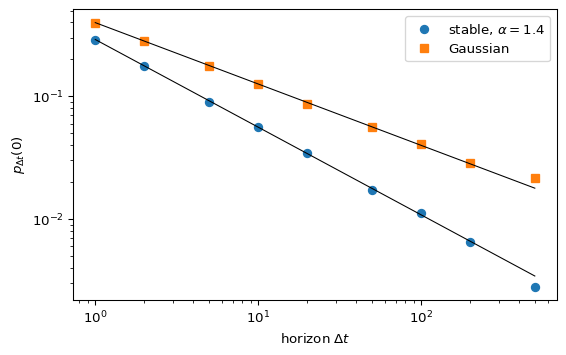
On log-log axes \(p_{\Delta t}(0)\) against \(\Delta t\) is a straight line with slope \(-1/\alpha\). For Gaussian returns \(\alpha = 2\) and the slope is \(-1/2\). The peak of the distribution is well sampled, so Equation 2 is easier to measure than the tail.
What Mantegna and Stanley found
(mantegna1995scaling?) used S&P 500 index values sampled every minute from 1984 to 1989. They report that:
- \(p_{\Delta t}(0)\) follows Equation 2 for \(\Delta t\) from 1 to 1000 minutes, three orders of magnitude.
- The slope is about \(-0.71\), which gives \(\alpha \approx 1.4\) (\(1.40 \pm 0.05\) in the paper). The exponent is stable over the six years of data.
- After rescaling with Equation 1, the central part of the distributions at different \(\Delta t\) matches a Lévy stable law.
- The far tails fall off faster than a Lévy law, approximately exponentially, so the variance is finite.
The last point led to the truncated Lévy flight: a Lévy flight whose largest steps are cut off. Sums of such steps look stable for a long range of \(n\) and only converge to a Gaussian after very many steps (mantegna1994stochastic?). Later work on the tails of individual US stocks found a power-law tail exponent close to 3, outside the stable range \(0 < \alpha \le 2\) (gopikrishnan1998inverse?). This is consistent with the heavy-tail and aggregational Gaussianity facts of Stylized Facts of Returns.
A simulated check
The figure applies the \(p_{\Delta t}(0)\) method to two synthetic series of \(10^6\) i.i.d. returns: symmetric stable with \(\alpha = 1.4\) and Gaussian. The density at zero is estimated as the fraction of aggregated returns in a window \(|r| < \varepsilon/2\) divided by \(\varepsilon\), with \(\varepsilon\) equal to one tenth of the interquartile range at that horizon.
Exercise
Fit the slope of \(\log p_{\Delta t}(0)\) against \(\log \Delta t\) for both series and convert it to an estimate of \(\alpha\). Then repeat the fit for the stable series using only \(\Delta t \ge 100\). Why does the estimate get noisier?
Solution
for label, r in series.items():
    p0 = np.array([p_zero(aggregate_returns(r, h)) for h in horizons])
    s_all = np.polyfit(np.log(horizons), np.log(p0), 1)[0]
    big = horizons >= 100
    s_big = np.polyfit(np.log(horizons[big]), np.log(p0[big]), 1)[0]
    name = label.replace("$", "").replace("\\alpha", "alpha")
    print(f"{name:18s} alpha (all) = {-1 / s_all:.2f}, alpha (dt >= 100) = {-1 / s_big:.2f}")
stable, alpha = 1.4 alpha (all) = 1.37, alpha (dt >= 100) = 1.15
Gaussian alpha (all) = 2.08, alpha (dt >= 100) = 2.52With \(10^6\) returns there are only 2000 non-overlapping blocks at \(\Delta t = 500\), and few of them fall inside the small window around zero. Long horizons cost data, which is why (mantegna1995scaling?) needed minute-by-minute prices to span three decades of \(\Delta t\).