Stylized Facts of Returns
Module 3: Modelling with Randomness
A stylized fact is a statistical property that appears in many markets, instruments and periods. (cont2001empirical?) lists eleven. Any model of prices should reproduce at least the first few. This page quotes the ones you test in the lab.
The facts you test in the lab
From (cont2001empirical?):
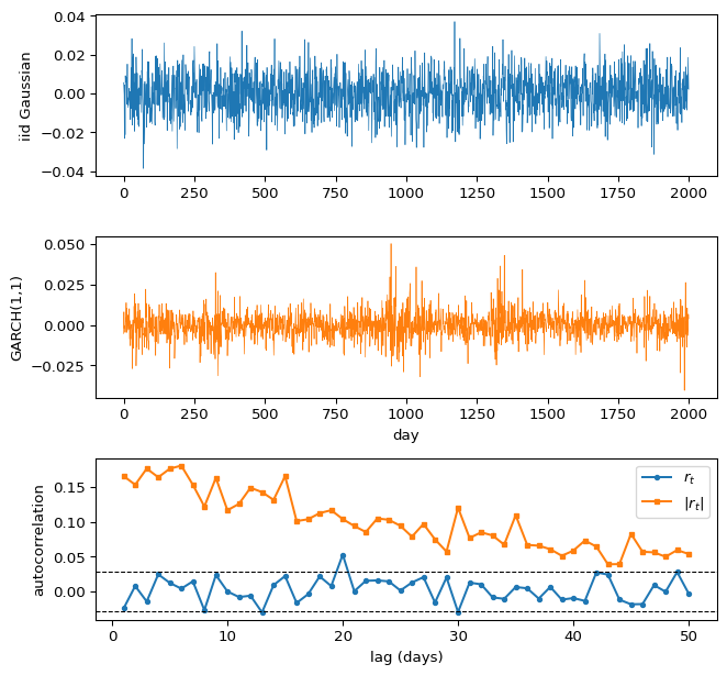
- Absence of autocorrelations. Linear autocorrelations of returns are often insignificant, except at very small intraday time scales (about 20 minutes).
- Heavy tails. The unconditional distribution of returns has a power-law or Pareto-like tail, with a tail index that is finite, higher than two and less than five for most data sets. This excludes both the normal distribution and stable laws with infinite variance.
- Aggregational Gaussianity. As the time scale \(\Delta t\) of the returns grows, their distribution looks more and more normal. The shape of the distribution is therefore not the same at different time scales.
- Volatility clustering. Measures of volatility have positive autocorrelation over several days: large changes tend to be followed by large changes, of either sign.
- Slow decay of autocorrelation in absolute returns. The autocorrelation of \(|r_t|\) decays roughly as a power law of the lag with an exponent between 0.2 and 0.4.
The list also contains gain/loss asymmetry, intermittency, conditional heavy tails, the leverage effect, volume/volatility correlation and asymmetry in time scales (cont2001empirical?).
What this does to the random walk model
The first fact supports the random walk hypothesis of Returns and Efficient Markets. The others reject its strong form. Uncorrelated is not the same as independent: \(|r_t|\) is predictable from \(|r_{t-1}|\) even when \(r_t\) is not predictable from \(r_{t-1}\) (cont2001empirical?). The heavy-tail fact also rejects Mandelbrot’s stable model with \(\alpha < 2\) (mandelbrot1963variation?) for the far tail, since a tail index above two means finite variance.
A model that reproduces some of them
The ARCH model of (engle1982autoregressive?) and its generalization GARCH(1,1) by (bollerslev1986generalized?) let the variance depend on the past:
\[ r_t = \sigma_t z_t, \qquad \sigma_t^2 = \omega + a\, r_{t-1}^2 + b\, \sigma_{t-1}^2 , \tag{1}\]
with \(z_t\) independent, zero mean and unit variance, and \(a + b < 1\) for a finite unconditional variance \(\omega / (1 - a - b)\). A large return raises tomorrow’s variance, which produces volatility clustering while \(r_t\) stays uncorrelated. See also (mantegna2000introduction?).
The figure compares i.i.d. Gaussian returns with a GARCH(1,1) series with Student-t innovations, the synthetic fallback of the lab (amlab.finance.synthetic_garch_prices). The GARCH series is built to show these facts, so the figure illustrates the definitions; it is not evidence about markets.
Exercise
Compute the excess kurtosis (scipy.stats.kurtosis) of the Gaussian and GARCH returns above. Then shuffle the GARCH returns in time with rng.permutation and recompute the autocorrelation of \(|r_t|\) at lag 1. Which property survives the shuffle, and which one disappears?
Solution
from scipy import stats

shuffled = rng.permutation(r_garch)
print(f"excess kurtosis, Gaussian: {stats.kurtosis(r_iid):.2f}")
print(f"excess kurtosis, GARCH:    {stats.kurtosis(r_garch):.2f}")
print(f"lag-1 ACF of |r|, GARCH:    {autocorrelation(np.abs(r_garch), 1)[1]:.3f}")
print(f"lag-1 ACF of |r|, shuffled: {autocorrelation(np.abs(shuffled), 1)[1]:.3f}")
excess kurtosis, Gaussian: 0.07
excess kurtosis, GARCH: 11.97
lag-1 ACF of |r|, GARCH: 0.166
lag-1 ACF of |r|, shuffled: -0.014Shuffling keeps the distribution, so the fat tails (large kurtosis) survive. It destroys the time order, so volatility clustering disappears. Heavy tails and clustering are separate facts, and a model can have one without the other.