Tail Exponent

Module 3: Modelling with Randomness

The normality tests told you that returns are not Gaussian. This page measures how heavy the tail is. You estimate the tail index $\alpha$ in $\Pr(|r| > x) \sim C x^{-\alpha}$ with the Hill estimator, and you compare it with the Gaussian ($\alpha = \infty$), with stable laws ($\alpha < 2$) and with the range $2 < \alpha < 5$ reported by (cont2001empirical?).

import matplotlib.pyplot as plt
import numpy as np

from amlab.finance import load_prices, log_returns

r = log_returns(load_prices()["close"])
a = np.abs(r - r.mean())

WARNING: data/finance/prices.csv not found. Using a SYNTHETIC GARCH(1,1) series with Student-t innovations (seed 2026). These are not market data. See data/finance/README.md.

Prediction

Exercise

Mandelbrot’s stable model predicts $\alpha < 2$ (mandelbrot1963variation?). A Gaussian has no power-law tail at all. Which value do you expect for your series? Write it down before you estimate it.

Solution

For market returns expect a value between 2 and 5, often close to 3 (cont2001empirical?; gopikrishnan1998inverse?). That is heavier than a Gaussian but lighter than a stable law. Compare your estimate with this range in the Interpretation section.

The Hill estimator

Sort the positive data in decreasing order, $X_{(1)} \ge X_{(2)} \ge \dots$. Using only the $k$ largest values,

\[ \hat{\alpha}_k = \left[ \frac{1}{k} \sum_{i=1}^{k} \ln \frac{X_{(i)}}{X_{(k+1)}} \right]^{-1} \tag{1}\]

(hill1975simple?). This is the power-law maximum likelihood estimator of Power Laws with $x_{\min} = X_{(k+1)}$, written for the CCDF exponent $\alpha = \alpha_{\text{pdf}} - 1$. For i.i.d. data with an exact power-law tail its standard error is approximately $\hat{\alpha}_k / \sqrt{k}$.

The choice of $k$ is a trade-off. Small $k$ uses few points and gives a noisy estimate. Large $k$ reaches into the centre of the distribution, where the power law does not hold, and biases the estimate. The usual tool is the Hill plot, $\hat{\alpha}_k$ against $k$: you look for a range of $k$ where it is roughly flat.

Core activity: implement and apply the estimator

Exercise

Implement Equation 1. Then apply it to the absolute returns a with $k = 100$.

def hill(x, k):
    """Hill estimate of the tail index from the k largest values of x > 0."""
    xs = # TODO: sort x in decreasing order
    # TODO: return 1 / mean(log(xs[:k] / xs[k]))
    return ...

Solution

def hill(x, k):
    """Hill estimate of the tail index from the k largest values of x > 0."""
    xs = np.sort(x)[::-1]
    return 1.0 / np.mean(np.log(xs[:k] / xs[k]))


print(f"k = 100: alpha = {hill(a, 100):.2f}")

k = 100: alpha = 3.28

A vectorized version that accepts an array of k values is amlab.finance.hill_estimator.

Validation on known tails

Before you trust the estimator on returns, apply it to samples whose tail index you know. A Student-t variable with $\nu$ degrees of freedom has $\Pr(|X| > x) \sim C x^{-\nu}$.

from amlab.finance import hill_estimator

rng = np.random.default_rng(31)
for nu in [2, 3, 4]:
    x = np.abs(rng.standard_t(nu, size=a.size))
    print(f"Student-t nu = {nu}: Hill (k = 100) = {hill_estimator(x, 100):.2f}")

Student-t nu = 2: Hill (k = 100) = 2.31
Student-t nu = 3: Hill (k = 100) = 3.01
Student-t nu = 4: Hill (k = 100) = 3.20

The estimates are close to $\nu$ but not equal. The Student-t tail is a power law only asymptotically, and the deviation grows with $\nu$. Keep this bias in mind when you read the value for returns.

Experiment: Hill plot

ks = np.arange(20, a.size // 5)
alpha_r = hill_estimator(a, ks)
gauss = np.abs(rng.normal(0.0, a.std(), a.size))
alpha_g = hill_estimator(gauss, ks)

fig, ax = plt.subplots(figsize=(7, 3.8))
ax.plot(ks, alpha_r, label="returns")
ax.fill_between(ks, alpha_r * (1 - 1 / np.sqrt(ks)), alpha_r * (1 + 1 / np.sqrt(ks)), alpha=0.2)
ax.plot(ks, alpha_g, label="Gaussian sample")
ax.axhspan(2, 5, color="grey", alpha=0.1, label="range in Cont (2001)")
ax.set_xscale("log")
ax.set_xlabel("number of upper order statistics $k$")
ax.set_ylabel(r"$\hat{\alpha}_k$")
ax.legend()
plt.tight_layout()
plt.show()

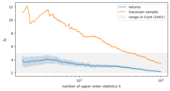
Figure 1: Hill plot of the absolute log returns and of a Gaussian sample of the same size and standard deviation. The shaded band is plus or minus one standard error $\hat{\alpha}_k/\sqrt{k}$ for the returns.

Interpretation

For heavy-tailed data the Hill plot has a plateau at small to intermediate $k$. For the Gaussian sample $\hat{\alpha}_k$ keeps growing as $k$ shrinks, because the true tail index is infinite: the estimator always returns a finite number, so the shape of the Hill plot matters more than any single value.

For market returns (cont2001empirical?) reports tail indices between 2 and 5, and (gopikrishnan1998inverse?) report values close to 3 for US stocks. A value above 2 means finite variance. Such a tail is heavy, but it is not the tail of a Lévy stable law with $\alpha < 2$.

Limitations

The standard error $\hat{\alpha}_k/\sqrt{k}$ assumes i.i.d. data. Volatility clustering makes the effective sample size smaller, so the real uncertainty is larger (cont2001empirical?).
A power law holds only asymptotically. A slowly varying correction, such as a logarithm, changes the estimate at every finite $k$ (cont2001empirical?).
There is no automatic rule for $k$ in this lab. Report the range of $k$ you used and show the Hill plot.

Optional extension

Exercise

Estimate the tail index separately for losses ($r < 0$) and gains ($r > 0$). Is there evidence for the gain/loss asymmetry listed by (cont2001empirical?)? Use the standard errors to judge whether the difference is larger than the noise.

Solution

Use the same $k$ for both tails. The standard error of the difference of two independent estimates is $\sqrt{s_1^2 + s_2^2}$. A smaller $\alpha$ for losses means a heavier loss tail. Call the asymmetry real only if the difference is about two standard errors or more, and check that it holds over a range of $k$.

rc = r - r.mean()
losses, gains = -rc[rc < 0], rc[rc > 0]
k = 100
a_loss, a_gain = hill_estimator(losses, k), hill_estimator(gains, k)
se = np.hypot(a_loss / np.sqrt(k), a_gain / np.sqrt(k))
print(f"losses {a_loss:.2f}, gains {a_gain:.2f}, difference {a_loss - a_gain:.2f} +/- {se:.2f}")

--- title: "Tail Exponent" subtitle: "Module 3: Modelling with Randomness" format: html --- The normality tests told you that returns are not Gaussian. This page measures *how* heavy the tail is. You estimate the tail index $\alpha$ in $\Pr(|r| > x) \sim C x^{-\alpha}$ with the Hill estimator, and you compare it with the Gaussian ($\alpha = \infty$), with stable laws ($\alpha < 2$) and with the range $2 < \alpha < 5$ reported by @cont2001empirical. ```{python} import matplotlib.pyplot as plt import numpy as np from amlab.finance import load_prices, log_returns r = log_returns(load_prices()["close"]) a = np.abs(r - r.mean()) ``` ## Prediction ::: {.callout-note} ## Exercise Mandelbrot's stable model predicts $\alpha < 2$ [@mandelbrot1963variation]. A Gaussian has no power-law tail at all. Which value do you expect for your series? Write it down before you estimate it. ::: ::: {.callout-tip collapse="true"} ## Solution For market returns expect a value between 2 and 5, often close to 3 [@cont2001empirical; @gopikrishnan1998inverse]. That is heavier than a Gaussian but lighter than a stable law. Compare your estimate with this range in the Interpretation section. ::: ## The Hill estimator Sort the positive data in decreasing order, $X_{(1)} \ge X_{(2)} \ge \dots$. Using only the $k$ largest values, $$ \hat{\alpha}_k = \left[ \frac{1}{k} \sum_{i=1}^{k} \ln \frac{X_{(i)}}{X_{(k+1)}} \right]^{-1} $$ {#eq-hill} [@hill1975simple]. This is the power-law maximum likelihood estimator of [Power Laws](power-laws.qmd) with $x_{\min} = X_{(k+1)}$, written for the CCDF exponent $\alpha = \alpha_{\text{pdf}} - 1$. For i.i.d. data with an exact power-law tail its standard error is approximately $\hat{\alpha}_k / \sqrt{k}$. The choice of $k$ is a trade-off. Small $k$ uses few points and gives a noisy estimate. Large $k$ reaches into the centre of the distribution, where the power law does not hold, and biases the estimate. The usual tool is the Hill plot, $\hat{\alpha}_k$ against $k$: you look for a range of $k$ where it is roughly flat. ## Core activity: implement and apply the estimator ::: {.callout-note} ## Exercise Implement @eq-hill. Then apply it to the absolute returns `a` with $k = 100$. ```python def hill(x, k): """Hill estimate of the tail index from the k largest values of x > 0.""" xs = # TODO: sort x in decreasing order # TODO: return 1 / mean(log(xs[:k] / xs[k])) return ... ``` ::: ::: {.callout-tip collapse="true"} ## Solution ```{python} def hill(x, k): """Hill estimate of the tail index from the k largest values of x > 0.""" xs = np.sort(x)[::-1] return 1.0 / np.mean(np.log(xs[:k] / xs[k])) print(f"k = 100: alpha = {hill(a, 100):.2f}") ``` A vectorized version that accepts an array of `k` values is `amlab.finance.hill_estimator`. ::: ## Validation on known tails Before you trust the estimator on returns, apply it to samples whose tail index you know. A Student-t variable with $\nu$ degrees of freedom has $\Pr(|X| > x) \sim C x^{-\nu}$. ```{python} from amlab.finance import hill_estimator rng = np.random.default_rng(31) for nu in [2, 3, 4]: x = np.abs(rng.standard_t(nu, size=a.size)) print(f"Student-t nu = {nu}: Hill (k = 100) = {hill_estimator(x, 100):.2f}") ``` The estimates are close to $\nu$ but not equal. The Student-t tail is a power law only asymptotically, and the deviation grows with $\nu$. Keep this bias in mind when you read the value for returns. ## Experiment: Hill plot ```{python} #| label: fig-lab-hill #| fig-cap: "Hill plot of the absolute log returns and of a Gaussian sample of the same size and standard deviation. The shaded band is plus or minus one standard error $\\hat{\\alpha}_k/\\sqrt{k}$ for the returns." ks = np.arange(20, a.size // 5) alpha_r = hill_estimator(a, ks) gauss = np.abs(rng.normal(0.0, a.std(), a.size)) alpha_g = hill_estimator(gauss, ks) fig, ax = plt.subplots(figsize=(7, 3.8)) ax.plot(ks, alpha_r, label="returns") ax.fill_between(ks, alpha_r * (1 - 1 / np.sqrt(ks)), alpha_r * (1 + 1 / np.sqrt(ks)), alpha=0.2) ax.plot(ks, alpha_g, label="Gaussian sample") ax.axhspan(2, 5, color="grey", alpha=0.1, label="range in Cont (2001)") ax.set_xscale("log") ax.set_xlabel("number of upper order statistics $k$") ax.set_ylabel(r"$\hat{\alpha}_k$") ax.legend() plt.tight_layout() plt.show() ``` ## Interpretation For heavy-tailed data the Hill plot has a plateau at small to intermediate $k$. For the Gaussian sample $\hat{\alpha}_k$ keeps growing as $k$ shrinks, because the true tail index is infinite: the estimator always returns a finite number, so the shape of the Hill plot matters more than any single value. For market returns @cont2001empirical reports tail indices between 2 and 5, and @gopikrishnan1998inverse report values close to 3 for US stocks. A value above 2 means finite variance. Such a tail is heavy, but it is not the tail of a Lévy stable law with $\alpha < 2$. ## Limitations - The standard error $\hat{\alpha}_k/\sqrt{k}$ assumes i.i.d. data. Volatility clustering makes the effective sample size smaller, so the real uncertainty is larger [@cont2001empirical]. - A power law holds only asymptotically. A slowly varying correction, such as a logarithm, changes the estimate at every finite $k$ [@cont2001empirical]. - There is no automatic rule for $k$ in this lab. Report the range of $k$ you used and show the Hill plot. ## Optional extension ::: {.callout-note} ## Exercise Estimate the tail index separately for losses ($r < 0$) and gains ($r > 0$). Is there evidence for the gain/loss asymmetry listed by @cont2001empirical? Use the standard errors to judge whether the difference is larger than the noise. ::: ::: {.callout-tip collapse="true"} ## Solution Use the same $k$ for both tails. The standard error of the difference of two independent estimates is $\sqrt{s_1^2 + s_2^2}$. A smaller $\alpha$ for losses means a heavier loss tail. Call the asymmetry real only if the difference is about two standard errors or more, and check that it holds over a range of $k$. ```python rc = r - r.mean() losses, gains = -rc[rc < 0], rc[rc > 0] k = 100 a_loss, a_gain = hill_estimator(losses, k), hill_estimator(gains, k) se = np.hypot(a_loss / np.sqrt(k), a_gain / np.sqrt(k)) print(f"losses {a_loss:.2f}, gains {a_gain:.2f}, difference {a_loss - a_gain:.2f} +/- {se:.2f}") ``` :::