C(0) = 0.600, formula 3(k-2)/(4(k-1)) = 0.600Module 5: Complex Networks
A random graph has short paths but almost no clustering. A regular lattice has high clustering but long paths. Watts and Strogatz built a one-parameter model that interpolates between the two (Watts and Strogatz 1998).
At \(p = 0\) you have the ring lattice. At \(p = 1\) you have a graph close to a random graph with the same number of edges. The degree distribution stays narrow for every \(p\): every node keeps at least \(k/2\) edges.
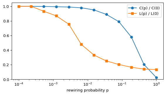
For the ring lattice, the clustering coefficient is \(C(0) = \frac{3(k-2)}{4(k-1)}\), which tends to \(3/4\) for large \(k\), and the average path length grows linearly with \(N\) (newman2003structure?). Watts and Strogatz found a wide range of small \(p\) in which \(L(p)\) has already dropped close to its random-graph value while \(C(p)\) is still close to \(C(0)\) (Watts and Strogatz 1998). A few random shortcuts are enough to shorten distances across the ring, while they destroy only a few triangles. Networks in this regime are called small-world networks. Watts and Strogatz reported the small-world property in a film actor collaboration network, the power grid of the western United States and the neural network of C. elegans (Watts and Strogatz 1998).
Figure 1 reproduces the shape of their Figure 2 on a smaller graph.
C(0) = 0.600, formula 3(k-2)/(4(k-1)) = 0.600In NetworkX, nx.watts_strogatz_graph(n, k, p) generates the model. The variant nx.connected_watts_strogatz_graph retries until the graph is connected, which you need to compute path lengths.
SEED = 7

G_sw = nx.watts_strogatz_graph(n=80, k=6, p=0.08, seed=SEED)
pos = nx.circular_layout(G_sw)
nx.draw(G_sw, pos=pos, node_size=40, node_color="lightblue", edge_color="gray")
plt.title("Watts-Strogatz graph, N = 80, k = 6, p = 0.08")
plt.show()

degrees = [d for _, d in G_sw.degree()]
print("degree range:", min(degrees), "to", max(degrees))
print(f"C = {nx.average_clustering(G_sw):.3f}")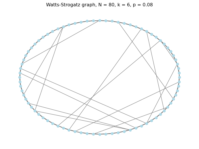
degree range: 4 to 7
C = 0.494
The circular layout keeps the ring visible, so you can spot the rewired shortcuts.
Compute \(C\) and \(L\) for nx.watts_strogatz_graph(80, 6, p) with \(p = 0\), \(p = 0.08\) and \(p = 1\). Which value of \(p\) gives a small-world network?
for p in [0, 0.08, 1]:
    G = nx.connected_watts_strogatz_graph(80, 6, p, seed=SEED)
    print(p, round(nx.average_clustering(G), 3), round(nx.average_shortest_path_length(G), 2))
At \(p = 0.08\) the clustering is still close to the lattice value (\(C(0) = 0.6\)), while \(L\) has dropped well below its lattice value. At \(p = 1\) both are close to random-graph values.
The model explains short paths together with high clustering. It does not produce hubs: for that you need preferential attachment.