Neither the random graph nor the small-world model produces hubs. Many real networks have heavy-tailed degree distributions, sometimes close to a power law \(p_k \sim k^{-\gamma}\)(Barabasi and Albert 1999; newman2003structure?). Barabási and Albert proposed that two ingredients generate such a distribution: growth and preferential attachment(Barabasi and Albert 1999).
The Barabási-Albert model
Start with a small network of \(m_0 \ge m\) nodes.
At each step add one new node with \(m\) edges.
Each new edge goes to an existing node \(i\) with probability proportional to its degree, \[
\Pi(k_i) = \frac{k_i}{\sum_j k_j}.
\]
Repeat until the network has \(N\) nodes.
The mean degree tends to \(\langle k \rangle = 2m\).
Key results
In the limit of large \(N\), the degree distribution is \[
p_k = \frac{2m(m+1)}{k(k+1)(k+2)} \sim k^{-3}, \qquad k \ge m,
\] so the exponent is \(\gamma = 3\)(newman2003structure?; Newman 2018).
The degrees of the oldest nodes grow like \(\sqrt{t}\), so the largest degree grows like \(k_{\max} \sim m\sqrt{N}\)(Barabasi and Albert 1999; Newman 2018).
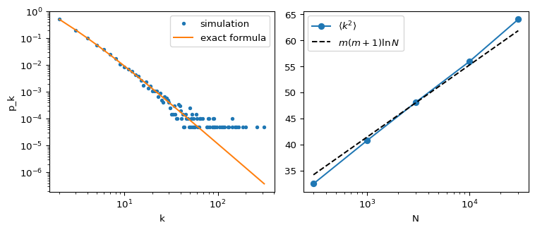
With \(\gamma = 3\) the second moment diverges logarithmically. Summing \(k^2 p_k\) up to \(k_{\max}\) gives \(\langle k^2 \rangle \approx m(m+1)\ln N\) for large \(N\). The degree variance\(\langle k^2 \rangle - \langle k \rangle^2\) therefore grows without bound as \(N\) grows, even though the mean stays at \(2m\).
The average path length is small, and the clustering is low and decreases with \(N\)(newman2003structure?).
The divergence of \(\langle k^2 \rangle\) drives two results of this module: the robustness to random failure in Robustness and Percolation and the vanishing epidemic threshold in Epidemic Threshold. Keep in mind that the divergence is slow: at realistic sizes \(\langle k^2 \rangle\) is large but finite.
Implementation
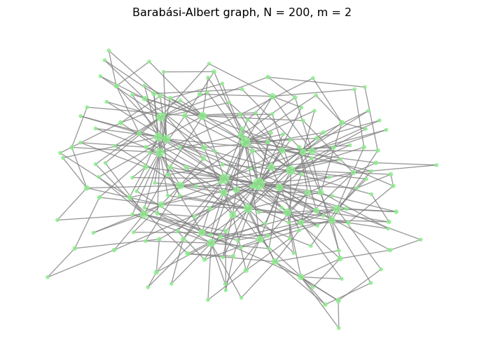
In NetworkX, nx.barabasi_albert_graph(n, m) adds nodes one at a time, each with m edges attached by preferential attachment.
import matplotlib.pyplot as pltimport networkx as nximport numpy as npSEED =7G_sf = nx.barabasi_albert_graph(n=200, m=2, seed=SEED)pos = nx.spring_layout(G_sf, seed=SEED)size = [5* d for _, d in G_sf.degree()]nx.draw(G_sf, pos=pos, node_size=size, node_color="lightgreen", edge_color="gray", alpha=0.8)plt.title("Barabási-Albert graph, N = 200, m = 2")plt.show()
Degree distribution and second moment
Figure 1 compares the empirical distribution with the exact formula. Use logarithmic bins or the complementary cumulative distribution for real data; here the formula lets you compare point by point.
Figure 1: Left: degree distribution of one Barabási-Albert graph (N = 20000, m = 2) against p_k = 2m(m+1)/(k(k+1)(k+2)). Right: second moment of the degree against N, with the approximation m(m+1) ln N (dashed).
The approximation \(m(m+1)\ln N\) follows the simulated values closely over two decades of \(N\). The small deviations come from the approximations in the sum (the lower limit \(k = m\) and the cutoff at \(k_{\max}\)) and from fluctuations of the largest degrees.
Exercise
Compute the mean and the variance of the degree for nx.barabasi_albert_graph(N, 2) with \(N = 10^3\) and \(N = 10^4\). Which one changes?
Solution
for N in [1_000, 10_000]: k = np.array([d for _, d in nx.barabasi_albert_graph(N, 2, seed=SEED).degree()])print(N, k.mean().round(2), k.var().round(1))
The mean stays close to \(2m = 4\). The variance grows with \(N\), as the logarithmic divergence of \(\langle k^2 \rangle\) predicts.
Other scale-free generators in NetworkX
nx.powerlaw_cluster_graph(n, m, p, seed=...) adds a triangle-closing step to preferential attachment, which raises the clustering.
nx.scale_free_graph(n, seed=...) returns a directed multigraph.
nx.configuration_model(degree_sequence, seed=...) builds a random graph with any degree sequence you choose.
For this course, nx.barabasi_albert_graph is usually the best starting point.
What’s Next?
The next page compares the three models with the same summary metrics.
Newman, Mark. 2018. Networks. 2nd ed. Oxford University Press.
Source Code
---title: "Preferential Attachment"subtitle: "Module 5: Complex Networks"format: html---Neither the random graph nor the small-world model produces hubs. Many real networks have heavy-tailed degree distributions, sometimes close to a power law $p_k \sim k^{-\gamma}$ [@barabasi1999emergence; @newman2003structure, Section 3.3]. Barabási and Albert proposed that two ingredients generate such a distribution: **growth** and **preferential attachment** [@barabasi1999emergence].## The Barabási-Albert model1. Start with a small network of $m_0 \ge m$ nodes.2. At each step add one new node with $m$ edges.3. Each new edge goes to an existing node $i$ with probability proportional to its degree, $$ \Pi(k_i) = \frac{k_i}{\sum_j k_j}. $$4. Repeat until the network has $N$ nodes.The mean degree tends to $\langle k \rangle = 2m$.## Key results- In the limit of large $N$, the degree distribution is $$ p_k = \frac{2m(m+1)}{k(k+1)(k+2)} \sim k^{-3}, \qquad k \ge m, $$ so the exponent is $\gamma = 3$ [@newman2003structure, Section 7.2; @newman2018networks].- The degrees of the oldest nodes grow like $\sqrt{t}$, so the largest degree grows like $k_{\max} \sim m\sqrt{N}$ [@barabasi1999emergence; @newman2018networks].- With $\gamma = 3$ the second moment diverges logarithmically. Summing $k^2 p_k$ up to $k_{\max}$ gives $\langle k^2 \rangle \approx m(m+1)\ln N$ for large $N$. The degree **variance** $\langle k^2 \rangle - \langle k \rangle^2$ therefore grows without bound as $N$ grows, even though the mean stays at $2m$.- The average path length is small, and the clustering is low and decreases with $N$ [@newman2003structure, Section 7.2].The divergence of $\langle k^2 \rangle$ drives two results of this module: the robustness to random failure in [Robustness and Percolation](robustness-percolation.qmd) and the vanishing epidemic threshold in [Epidemic Threshold](epidemic-threshold.qmd). Keep in mind that the divergence is slow: at realistic sizes $\langle k^2 \rangle$ is large but finite.## ImplementationIn NetworkX, `nx.barabasi_albert_graph(n, m)` adds nodes one at a time, each with `m` edges attached by preferential attachment.```{python}import matplotlib.pyplot as pltimport networkx as nximport numpy as npSEED =7G_sf = nx.barabasi_albert_graph(n=200, m=2, seed=SEED)pos = nx.spring_layout(G_sf, seed=SEED)size = [5* d for _, d in G_sf.degree()]nx.draw(G_sf, pos=pos, node_size=size, node_color="lightgreen", edge_color="gray", alpha=0.8)plt.title("Barabási-Albert graph, N = 200, m = 2")plt.show()```## Degree distribution and second moment@fig-ba-degree compares the empirical distribution with the exact formula. Use logarithmic bins or the complementary cumulative distribution for real data; here the formula lets you compare point by point.```{python}#| label: fig-ba-degree#| fig-cap: "Left: degree distribution of one Barabási-Albert graph (N = 20000, m = 2) against p_k = 2m(m+1)/(k(k+1)(k+2)). Right: second moment of the degree against N, with the approximation m(m+1) ln N (dashed)."#| echo: falsem =2G = nx.barabasi_albert_graph(20_000, m, seed=SEED)deg = np.array([d for _, d in G.degree()])ks, counts = np.unique(deg, return_counts=True)fig, axes = plt.subplots(1, 2, figsize=(8, 3.5))axes[0].loglog(ks, counts / counts.sum(), "o", ms=3, label="simulation")k_th = np.arange(m, ks.max() +1)axes[0].loglog(k_th, 2* m * (m +1) / (k_th * (k_th +1) * (k_th +2)), label="exact formula")axes[0].set_xlabel("k")axes[0].set_ylabel("p_k")axes[0].legend()Ns = np.array([300, 1000, 3000, 10_000, 30_000])k2 = [np.mean(np.array([d for _, d in nx.barabasi_albert_graph(n, m, seed=SEED).degree()]) **2) for n in Ns]axes[1].semilogx(Ns, k2, "o-", label=r"$\langle k^2 \rangle$")axes[1].semilogx(Ns, m * (m +1) * np.log(Ns), "k--", label=r"$m(m+1)\ln N$")axes[1].set_xlabel("N")axes[1].legend()plt.tight_layout()plt.show()```The approximation $m(m+1)\ln N$ follows the simulated values closely over two decades of $N$. The small deviations come from the approximations in the sum (the lower limit $k = m$ and the cutoff at $k_{\max}$) and from fluctuations of the largest degrees.::: {.callout-note}## ExerciseCompute the mean and the variance of the degree for `nx.barabasi_albert_graph(N, 2)` with $N = 10^3$ and $N = 10^4$. Which one changes?:::::: {.callout-tip collapse="true"}## Solution```pythonfor N in [1_000, 10_000]: k = np.array([d for _, d in nx.barabasi_albert_graph(N, 2, seed=SEED).degree()])print(N, k.mean().round(2), k.var().round(1))```The mean stays close to $2m = 4$. The variance grows with $N$, as the logarithmic divergence of $\langle k^2 \rangle$ predicts.:::::: {.callout-tip collapse="true"}## Other scale-free generators in NetworkX- `nx.powerlaw_cluster_graph(n, m, p, seed=...)` adds a triangle-closing step to preferential attachment, which raises the clustering.- `nx.scale_free_graph(n, seed=...)` returns a directed multigraph.- `nx.configuration_model(degree_sequence, seed=...)` builds a random graph with any degree sequence you choose.For this course, `nx.barabasi_albert_graph` is usually the best starting point.:::## What's Next?The next page compares the three models with the same summary metrics.[Comparing Graph Models](comparing-models.qmd){.btn .btn-primary}