Mean Squared Displacement
Module 3: Modelling with Randomness
The mean squared displacement (MSD) measures how far a random walker spreads. It is the standard quantity you compute from tracked particles, cells or animals.
Definition
For an ensemble of walkers that start at the origin,
\[ \mathrm{MSD}(t) = \langle |\mathbf{x}(t) - \mathbf{x}(0)|^2 \rangle , \]
where \(\langle \cdot \rangle\) is the average over walkers. For the unbiased 1D lattice walk you found \(\langle x^2(n) \rangle = n\delta^2\) in The Random Walk.
Diffusive scaling
A walker that takes one step every \(\tau\) seconds has made \(n = t/\tau\) steps at time \(t\). Then \(\langle x^2 \rangle = (t/\tau)\,\delta^2\). (berg1993random?, Eqs. 1.9 to 1.11) defines the diffusion coefficient
\[ D = \frac{\delta^2}{2\tau} \tag{1}\]
and obtains
\[ \langle x^2(t) \rangle = 2Dt . \tag{2}\]
Motions along different axes are independent, so each coordinate contributes \(2Dt\). In \(d\) dimensions
\[ \langle r^2(t) \rangle = 2dDt , \tag{3}\]
which gives \(4Dt\) in the plane and \(6Dt\) in space (berg1993random?, Eqs. 1.13 and 1.14). The root-mean-square distance grows as \(\sqrt{t}\). To go twice as far, a diffusing particle needs four times as long.
A simulated check
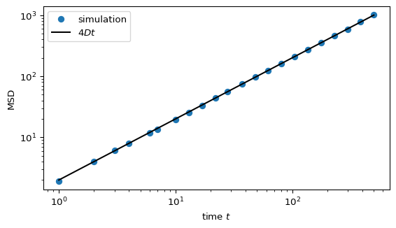
The figure uses 2000 planar walkers with independent Gaussian steps of standard deviation \(\sigma = 1\) per coordinate and \(\tau = 1\). Each coordinate has step variance \(\sigma^2\), so \(D = \sigma^2 / (2\tau) = 1/2\) and Equation 3 predicts \(\mathrm{MSD} = 4Dt = 2t\).
Anomalous diffusion
Many experiments find \(\mathrm{MSD} \propto t^{\gamma}\) with \(\gamma \neq 1\). The case \(\gamma < 1\) is subdiffusion and \(\gamma > 1\) is superdiffusion (metzler2000random?). Such behaviour requires that one of the random walk assumptions fails: steps are correlated, waiting times have no finite mean, or step lengths have no finite variance. You see the last case in Lévy flights.
Exercise
Estimate \(D\) from the simulation by fitting a straight line to \(\mathrm{MSD}(t)\) through the origin. How close is your estimate to \(1/2\)? Then fit the exponent \(\gamma\) as the slope of \(\log \mathrm{MSD}\) against \(\log t\).
Solution
The least-squares slope through the origin is \(\sum t\,\mathrm{MSD} / \sum t^2\), and \(D\) is that slope divided by \(2d = 4\).
slope = np.sum(t * msd) / np.sum(t**2)
gamma = np.polyfit(np.log(t[1:]), np.log(msd[1:]), 1)[0]
print(f"D estimate: {slope / 4:.3f}  (theory 0.5)")
print(f"exponent gamma: {gamma:.3f}  (theory 1)")
D estimate: 0.504 (theory 0.5)
exponent gamma: 1.007 (theory 1)