Unstable Modes in 2D

Module 4: Space and Pattern Formation

In 1D you scanned the Neumann modes $n$. On a rectangle the modes are pairs $(n, m)$ (murray2003mathematical?). This page extends the scan and compares it with the 2D simulation.

Modes on a Rectangle

With Neumann boundaries on $[0, L_x] \times [0, L_y]$ (see Laplacian Eigenmodes),

\[ k_{n,m}^2 = \left(\frac{n\pi}{L_x}\right)^2 + \left(\frac{m\pi}{L_y}\right)^2, \qquad A_{n,m} = \gamma J - k_{n,m}^2\,\mathrm{diag}(1, d). \tag{1}\]

Mode $(n, 0)$ varies only in $x$ and $(0, m)$ only in $y$; both are stripes. Modes with $n, m \ge 1$ are checkerboards of spots. For periodic boundaries replace $\pi/L$ by $2\pi/L$.

Extend the Mode Scan

Exercise

Extend your 1D scan to mode pairs $(n, m)$. Skip the flat mode $(0, 0)$.

import numpy as np

def find_unstable_modes_2d(a=0.40, b=1.00, d=30.0, gamma=1.0, length_x=20.0, length_y=50.0, num_modes=12):
    jac = np.array(gierer_meinhardt_jacobian(a, b)).reshape(2, 2)
    diffusion = np.diag([1.0, d])
    unstable_modes = []

    for n in range(num_modes):
        for m in range(num_modes):
            if n == 0 and m == 0:
                continue
            # TODO: compute k2 and A_nm
            # TODO: store ((n, m), growth_rate) if the growth rate is positive

    unstable_modes.sort(key=lambda item: item[1], reverse=True)
    return unstable_modes

Solution

def find_unstable_modes_2d(a=0.40, b=1.00, d=30.0, gamma=1.0, length_x=20.0, length_y=50.0, num_modes=12):
    jac = np.array(gierer_meinhardt_jacobian(a, b)).reshape(2, 2)
    diffusion = np.diag([1.0, d])
    unstable_modes = []

    for n in range(num_modes):
        for m in range(num_modes):
            if n == 0 and m == 0:
                continue
            k2 = (n * np.pi / length_x) ** 2 + (m * np.pi / length_y) ** 2
            a_nm = gamma * jac - k2 * diffusion
            growth_rate = np.max(np.linalg.eigvals(a_nm).real)
            if growth_rate > 0:
                unstable_modes.append(((n, m), growth_rate))

    unstable_modes.sort(key=lambda item: item[1], reverse=True)
    return unstable_modes

Compare Case A and Case B

Exercise

Use your functions with $a = 0.40$, $b = 1.00$ on $L_x = 20$, $L_y = 50$, for $d = 30$ (Case A) and $d = 20$ (Case B).

Does each case satisfy the Turing conditions?
How many unstable mode pairs $(n, m)$ appear on the rectangle?
What is the dominant mode pair?

Then run the simulation for each case and check whether the observed stripes or spots match the dominant mode.

Solution

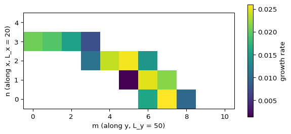
Case A satisfies the Turing conditions and has 14 unstable mode pairs. The dominant pair is the stripe $(0, 7)$. Case B fails the conditions and has none. The reference implementation gives the same list.

from amlab.turing import unstable_modes_2d

for label, d in (("Case A", 30.0), ("Case B", 20.0)):
    modes = unstable_modes_2d(a=0.40, b=1.00, d=d, length_x=20.0, length_y=50.0)
    print(f"{label}: {len(modes)} unstable modes")
    for (n, m), rate in modes[:5]:
        print(f"   (n, m) = ({n}, {m})   growth rate = {rate:.4f}")

Case A: 14 unstable modes
   (n, m) = (0, 7)   growth rate = 0.0259
   (n, m) = (2, 5)   growth rate = 0.0255
   (n, m) = (1, 6)   growth rate = 0.0248
   (n, m) = (2, 4)   growth rate = 0.0237
   (n, m) = (1, 7)   growth rate = 0.0216
Case B: 0 unstable modes

Figure 1: Growth rate of each Neumann mode $(n, m)$ for Case A on $L_x = 20$, $L_y = 50$. Only positive rates are coloured.

Case B has no unstable mode, as in 1D. Case A has many, and the top few have almost the same rate: the stripe $(0, 7)$ and the spot modes $(2, 5)$ and $(1, 6)$ differ by less than 5%. Linear theory alone cannot tell you which one wins. In the simulation on Gierer-Meinhardt Solver in 2D, the nonlinear terms select spots. This is a limitation of the linear analysis: it predicts the unstable band and the spacing, not the final shape (murray2003mathematical?).

Warning

amlab.pdes_2d.find_unstable_spatial_modes skips the stripe modes with $n = 0$ or $m = 0$, and returns every scanned mode when none is unstable. Use amlab.turing.unstable_modes_2d for the analysis.

Exercise

Estimate the spot spacing from the growth-rate peak. The fastest continuous wavenumber for Case A is $k_{\max} \approx 0.43$. What wavelength does that give, and how does it compare with the distance between neighbouring spots in the simulation?

Solution

The wavelength is $2\pi/0.43 \approx 14.6$. In the snapshot neighbouring spots in the same row are about $28$ apart along $y$, and rows are offset by half that distance, so nearest neighbours sit at a distance of roughly $16$ to $18$, slightly above the linear wavelength. The spacing is close to the linear wavelength even though the arrangement is chosen by the nonlinear terms.

--- title: "Unstable Modes in 2D" subtitle: "Module 4: Space and Pattern Formation" format: html --- In 1D you scanned the Neumann modes $n$. On a rectangle the modes are pairs $(n, m)$ [@murray2003mathematical, Section 2.5]. This page extends the scan and compares it with the 2D simulation. ## Modes on a Rectangle With Neumann boundaries on $[0, L_x] \times [0, L_y]$ (see [Laplacian Eigenmodes](laplacian-eigenmodes.qmd)), $$ k_{n,m}^2 = \left(\frac{n\pi}{L_x}\right)^2 + \left(\frac{m\pi}{L_y}\right)^2, \qquad A_{n,m} = \gamma J - k_{n,m}^2\,\mathrm{diag}(1, d). $$ {#eq-gm2m-modes} Mode $(n, 0)$ varies only in $x$ and $(0, m)$ only in $y$; both are stripes. Modes with $n, m \ge 1$ are checkerboards of spots. For periodic boundaries replace $\pi/L$ by $2\pi/L$. ## Extend the Mode Scan ::: {.callout-note} ## Exercise Extend your 1D scan to mode pairs $(n, m)$. Skip the flat mode $(0, 0)$. ```python import numpy as np def find_unstable_modes_2d(a=0.40, b=1.00, d=30.0, gamma=1.0, length_x=20.0, length_y=50.0, num_modes=12): jac = np.array(gierer_meinhardt_jacobian(a, b)).reshape(2, 2) diffusion = np.diag([1.0, d]) unstable_modes = [] for n in range(num_modes): for m in range(num_modes): if n == 0 and m == 0: continue # TODO: compute k2 and A_nm # TODO: store ((n, m), growth_rate) if the growth rate is positive unstable_modes.sort(key=lambda item: item[1], reverse=True) return unstable_modes ``` ::: ::: {.callout-tip collapse="true"} ## Solution ```python def find_unstable_modes_2d(a=0.40, b=1.00, d=30.0, gamma=1.0, length_x=20.0, length_y=50.0, num_modes=12): jac = np.array(gierer_meinhardt_jacobian(a, b)).reshape(2, 2) diffusion = np.diag([1.0, d]) unstable_modes = [] for n in range(num_modes): for m in range(num_modes): if n == 0 and m == 0: continue k2 = (n * np.pi / length_x) ** 2 + (m * np.pi / length_y) ** 2 a_nm = gamma * jac - k2 * diffusion growth_rate = np.max(np.linalg.eigvals(a_nm).real) if growth_rate > 0: unstable_modes.append(((n, m), growth_rate)) unstable_modes.sort(key=lambda item: item[1], reverse=True) return unstable_modes ``` ::: ## Compare Case A and Case B ::: {.callout-note} ## Exercise Use your functions with $a = 0.40$, $b = 1.00$ on $L_x = 20$, $L_y = 50$, for $d = 30$ (Case A) and $d = 20$ (Case B). - Does each case satisfy the Turing conditions? - How many unstable mode pairs $(n, m)$ appear on the rectangle? - What is the dominant mode pair? Then run the simulation for each case and check whether the observed stripes or spots match the dominant mode. ::: ::: {.callout-tip collapse="true"} ## Solution Case A satisfies the Turing conditions and has 14 unstable mode pairs. The dominant pair is the stripe $(0, 7)$. Case B fails the conditions and has none. The reference implementation gives the same list. ```{python} from amlab.turing import unstable_modes_2d for label, d in (("Case A", 30.0), ("Case B", 20.0)): modes = unstable_modes_2d(a=0.40, b=1.00, d=d, length_x=20.0, length_y=50.0) print(f"{label}: {len(modes)} unstable modes") for (n, m), rate in modes[:5]: print(f" (n, m) = ({n}, {m}) growth rate = {rate:.4f}") ``` ::: ```{python} #| label: fig-gm2m-rates #| fig-cap: 'Growth rate of each Neumann mode $(n, m)$ for Case A on $L_x = 20$, $L_y = 50$. Only positive rates are coloured.' #| fig-width: 7 #| fig-height: 3 #| echo: false import matplotlib.pyplot as plt import numpy as np from amlab.turing import dispersion_relation, gierer_meinhardt_jacobian jac = gierer_meinhardt_jacobian(0.40, 1.00) n = np.arange(5) m = np.arange(11) k2 = (n[:, None] * np.pi / 20) ** 2 + (m[None, :] * np.pi / 50) ** 2 rates = dispersion_relation(k2, *jac, 30.0) rates[0, 0] = np.nan fig, ax = plt.subplots(figsize=(7, 3)) im = ax.imshow(np.where(rates > 0, rates, np.nan), origin="lower", cmap="viridis") ax.set_xlabel("m (along y, L_y = 50)") ax.set_ylabel("n (along x, L_x = 20)") plt.colorbar(im, ax=ax, label="growth rate") plt.show() plt.close() ``` Case B has no unstable mode, as in 1D. Case A has many, and the top few have almost the same rate: the stripe $(0, 7)$ and the spot modes $(2, 5)$ and $(1, 6)$ differ by less than 5%. Linear theory alone cannot tell you which one wins. In the simulation on [Gierer-Meinhardt Solver in 2D](gierer-meinhardt-2d-solver.qmd), the nonlinear terms select spots. This is a limitation of the linear analysis: it predicts the unstable band and the spacing, not the final shape [@murray2003mathematical, Section 2.6]. ::: {.callout-warning} `amlab.pdes_2d.find_unstable_spatial_modes` skips the stripe modes with $n = 0$ or $m = 0$, and returns every scanned mode when none is unstable. Use `amlab.turing.unstable_modes_2d` for the analysis. ::: ::: {.callout-note} ## Exercise Estimate the spot spacing from the growth-rate peak. The fastest continuous wavenumber for Case A is $k_{\max} \approx 0.43$. What wavelength does that give, and how does it compare with the distance between neighbouring spots in the simulation? ::: ::: {.callout-tip collapse="true"} ## Solution The wavelength is $2\pi/0.43 \approx 14.6$. In the snapshot neighbouring spots in the same row are about $28$ apart along $y$, and rows are offset by half that distance, so nearest neighbours sit at a distance of roughly $16$ to $18$, slightly above the linear wavelength. The spacing is close to the linear wavelength even though the arrangement is chosen by the nonlinear terms. :::