Laplacian Eigenmodes
Module 4: Space and Pattern Formation
The linearized system \(\partial_t \eta = D\,\Delta\eta + \gamma J\eta\) couples every point to its neighbours. You decouple it by expanding \(\eta\) in eigenfunctions of the Laplacian, which depend on the domain and the boundary conditions (murray2003mathematical?; britton2003essential?).
The Eigenvalue Problem
Look for functions \(\phi\) and numbers \(k^2 \ge 0\) with
\[ \Delta \phi + k^2 \phi = 0 \quad \text{in } \Omega, \tag{1}\]
plus the boundary condition of the model. The eigenvalue of \(\Delta\) is \(\lambda = -k^2\), and \(k\) is the wavenumber. The wavelength of the mode is \(2\pi / k\).
On an Interval \((0, L)\)
| Boundary condition | Condition | Eigenfunctions | Wavenumbers |
|---|---|---|---|
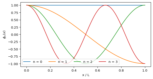
| Neumann (zero flux) | \(\phi'(0) = \phi'(L) = 0\) | \(\cos(n\pi x / L)\) | \(k_n = n\pi/L\), \(n = 0, 1, 2, \dots\) |
| Dirichlet (fixed value) | \(\phi(0) = \phi(L) = 0\) | \(\sin(n\pi x / L)\) | \(k_n = n\pi/L\), \(n = 1, 2, \dots\) |
| Periodic | \(\phi(0) = \phi(L)\), \(\phi'(0) = \phi'(L)\) | \(\cos(2n\pi x/L)\), \(\sin(2n\pi x/L)\) | \(k_n = 2n\pi/L\), \(n = 0, 1, 2, \dots\) |
Mode \(n\) with Neumann conditions fits \(n\) half-wavelengths into the interval. Mode \(0\) is the flat perturbation. For periodic conditions each \(n \ge 1\) has two independent eigenfunctions with the same \(k_n\).
On a Rectangle \((0, L_x) \times (0, L_y)\)
Separation of variables gives products of the 1D eigenfunctions. With Neumann conditions on all four edges,
\[ \phi_{n,m}(x, y) = \cos\left(\frac{n\pi x}{L_x}\right)\cos\left(\frac{m\pi y}{L_y}\right), \qquad k_{n,m}^2 = \left(\frac{n\pi}{L_x}\right)^2 + \left(\frac{m\pi}{L_y}\right)^2. \tag{2}\]
For Dirichlet conditions replace cosines by sines and start at \(n, m \ge 1\). For periodic conditions replace \(\pi/L\) by \(2\pi/L\). Different pairs \((n, m)\) can share almost the same \(k^2\). That is why 2D domains can select stripes, spots, or mixtures (murray2003mathematical?).
Mode Decomposition
Expand the perturbation as
\[ \eta(x, t) = \sum_n c_n(t)\,\phi_n(x), \qquad c_n(t) \in \mathbb{R}^2. \]
Because \(\Delta \phi_n = -k_n^2 \phi_n\), the modes separate and each coefficient solves a \(2 \times 2\) linear ODE:
\[ \dot c_n = A_n c_n, \qquad A_n = \gamma J - k_n^2 D. \tag{3}\]
So \(c_n(t) \propto e^{\sigma t}\), where \(\sigma\) is an eigenvalue of \(A_n\). The uniform state is linearly stable when every admissible mode has \(\operatorname{Re}\sigma < 0\). The next session turns this into the Turing conditions and the dispersion relation.
Exercise
On \((0, 40)\) with Neumann conditions, which mode \(n\) has wavenumber closest to \(k = 0.4\)? How many half-wavelengths does it fit into the domain?
Solution
\(k_n = n\pi/40\), so \(n = 40k/\pi \approx 5.09\). The closest mode is \(n = 5\), with five half-wavelengths, which is two and a half full wavelengths.
Next session: Turing Conditions.