Time-Step Stability

Module 4: Space and Pattern Formation

Explicit Euler is simple, but it is only conditionally stable for diffusion. If $dt$ is too large for the grid, the simulation produces a pattern that is not in the PDE and then overflows. This page derives the bound, shows the artefact, and gives a convergence check you should run before trusting any reaction-diffusion figure (leveque2007finite?).

The Stability Bound in 1D

Apply explicit Euler and the 3-point Laplacian to pure diffusion $u_t = D\,u_{xx}$:

\[ u_j^{n+1} = u_j^n + r\left(u_{j+1}^n - 2u_j^n + u_{j-1}^n\right), \qquad r = \frac{D\,dt}{dx^2}. \]

Insert a Fourier mode $u_j^n = G^n e^{i k j\,dx}$ (von Neumann analysis). The amplification factor per step is

\[ G(k) = 1 - 4r\sin^2\left(\frac{k\,dx}{2}\right). \tag{1}\]

The scheme is stable when $|G| \le 1$ for every $k$. The worst case is the grid-scale sawtooth $k = \pi/dx$, where $G = 1 - 4r$. Requiring $1 - 4r \ge -1$ gives

\[ dt \le \frac{dx^2}{2D} \quad \text{(1D)}. \tag{2}\]

The Bound in 2D

With the 5-point stencil, the same argument gives $G = 1 - 4r\left[\sin^2(k_x dx/2) + \sin^2(k_y dx/2)\right]$. The worst mode is the checkerboard, with $G = 1 - 8r$, so

\[ dt \le \frac{dx^2}{4D} \quad \text{(2D, 5-point stencil)}. \tag{3}\]

For a system, use the largest diffusion coefficient. In the Gierer-Meinhardt scaling that is $d$. The reaction terms add a further, usually weaker, restriction (leveque2007finite?).

from amlab.turing import euler_dt_max

settings = [
    ("GM 1D, d = 30, dx = 1", 1.0, 30.0, 1, 0.01),
    ("GM 1D, d = 30, dx = 0.5", 0.5, 30.0, 1, 0.001),
    ("GM 2D, d = 30, dx = 1", 1.0, 30.0, 2, 0.005),
    ("Gray-Scott 2D, D1 = 0.1, dx = 1", 1.0, 0.1, 2, 2.0),
]
for label, dx, diff, ndim, dt in settings:
    bound = euler_dt_max(dx, diff, ndim)
    print(f"{label:34s} bound = {bound:.5f}   dt used = {dt:<6} ok: {dt <= bound}")

GM 1D, d = 30, dx = 1              bound = 0.01667   dt used = 0.01   ok: True
GM 1D, d = 30, dx = 0.5            bound = 0.00417   dt used = 0.001  ok: True
GM 2D, d = 30, dx = 1              bound = 0.00833   dt used = 0.005  ok: True
Gray-Scott 2D, D1 = 0.1, dx = 1    bound = 2.50000   dt used = 2.0    ok: True

A Numerical Artefact

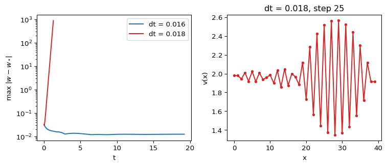
Figure 1 runs Case A ($d = 30$, $dx = 1$), where the bound is $1/60 \approx 0.0167$, with $dt = 0.016$ and $dt = 0.018$.

Figure 1: Left: maximum deviation from the steady state for two time steps. Right: profile of $v$ for $dt = 0.018$ after 25 steps, showing the grid-scale sawtooth that the PDE does not contain.

With $dt = 0.016$ the noise decays within a few time units and the deviation then stays small. The Turing mode grows only at rate $\sigma \approx 0.02$, so it becomes visible on longer runs. With $dt = 0.018$ the deviation grows by a fixed factor per step, close to $|1 - 4r| = 1.16$, and the profile alternates up and down between neighbouring points. That sawtooth is the signature of a violated stability bound. Do not interpret it as a pattern.

A Convergence Check

A stable run can still be inaccurate. To check, refine the grid and compare. The Laplacian error is $\mathcal{O}(dx^2)$ and the Euler error is $\mathcal{O}(dt)$.

Refining is subtle: if you halve $dx$ and only halve $dt$, the ratio $dt/dx^2$ doubles and you can cross the bound. Starting from $dx = 1$, $dt = 0.01$, halving both gives $dt = 0.005 > 0.25/60$, which is unstable. Divide $dt$ by four whenever you halve $dx$.

The check below uses periodic boundaries and a smooth initial perturbation, so the coarse grid points are a subset of the fine ones. It compares successive refinements $e_1 = \max|w_h - w_{h/2}|$ and $e_2 = \max|w_{h/2} - w_{h/4}|$ at $t = 50$. The observed order is $p = \log_2(e_1/e_2)$.

import numpy as np

from amlab.turing import simulate_gm_1d


def smooth_start(x, length=40.0):
    mode3 = np.cos(6 * np.pi * x / length)
    return 0.01 * np.array([mode3 + 0.5 * np.cos(10 * np.pi * x / length), mode3])


def run(dx, dt):
    return simulate_gm_1d(d=30.0, dx=dx, dt=dt, t_end=50.0, bc="periodic", initial=smooth_start)[1]


space = [run(1.0, 0.01), run(0.5, 0.0025), run(0.25, 0.000625)]
e1 = np.max(np.abs(space[0] - space[1][:, ::2]))
e2 = np.max(np.abs(space[1] - space[2][:, ::2]))
print(f"space and time (dx halved, dt / 4): e1 = {e1:.2e}, e2 = {e2:.2e}, p = {np.log2(e1 / e2):.2f}")

time = [run(1.0, 0.01), run(1.0, 0.005), run(1.0, 0.0025)]
e1 = np.max(np.abs(time[0] - time[1]))
e2 = np.max(np.abs(time[1] - time[2]))
print(f"time only (dx = 1, dt halved):     e1 = {e1:.2e}, e2 = {e2:.2e}, p = {np.log2(e1 / e2):.2f}")

space and time (dx halved, dt / 4): e1 = 1.53e-03, e2 = 3.91e-04, p = 1.97
time only (dx = 1, dt halved):     e1 = 2.23e-06, e2 = 1.11e-06, p = 1.00

The first line gives $p \approx 2$, the expected second order. The second gives $p \approx 1$, the order of explicit Euler. The time error at $dt = 0.01$ is much smaller than the space error at $dx = 1$, so for this problem $dx$ controls the accuracy. In your own work, report both checks.

Exercise

You run Gierer-Meinhardt in 2D with $d = 30$ and $dx = 1$. What is the largest stable $dt$? Would $dt = 0.01$, which is safe in 1D, work?

Solution

The 2D bound is $dx^2/(4d) = 1/120 \approx 0.0083$. So $dt = 0.01$ is unstable in 2D, even though it is stable in 1D. The 2D solver page uses $dt = 0.005$ and $dt = 0.008$.

--- title: "Time-Step Stability" subtitle: "Module 4: Space and Pattern Formation" format: html --- Explicit Euler is simple, but it is only conditionally stable for diffusion. If $dt$ is too large for the grid, the simulation produces a pattern that is not in the PDE and then overflows. This page derives the bound, shows the artefact, and gives a convergence check you should run before trusting any reaction-diffusion figure [@leveque2007finite, Chapter 9]. ## The Stability Bound in 1D Apply explicit Euler and the 3-point Laplacian to pure diffusion $u_t = D\,u_{xx}$: $$ u_j^{n+1} = u_j^n + r\left(u_{j+1}^n - 2u_j^n + u_{j-1}^n\right), \qquad r = \frac{D\,dt}{dx^2}. $$ Insert a Fourier mode $u_j^n = G^n e^{i k j\,dx}$ (von Neumann analysis). The amplification factor per step is $$ G(k) = 1 - 4r\sin^2\left(\frac{k\,dx}{2}\right). $$ {#eq-ts-amplification} The scheme is stable when $|G| \le 1$ for every $k$. The worst case is the grid-scale sawtooth $k = \pi/dx$, where $G = 1 - 4r$. Requiring $1 - 4r \ge -1$ gives $$ dt \le \frac{dx^2}{2D} \quad \text{(1D)}. $$ {#eq-ts-bound-1d} ## The Bound in 2D With the 5-point stencil, the same argument gives $G = 1 - 4r\left[\sin^2(k_x dx/2) + \sin^2(k_y dx/2)\right]$. The worst mode is the checkerboard, with $G = 1 - 8r$, so $$ dt \le \frac{dx^2}{4D} \quad \text{(2D, 5-point stencil)}. $$ {#eq-ts-bound-2d} For a system, use the largest diffusion coefficient. In the Gierer-Meinhardt scaling that is $d$. The reaction terms add a further, usually weaker, restriction [@leveque2007finite, Chapter 9]. ```{python} from amlab.turing import euler_dt_max settings = [ ("GM 1D, d = 30, dx = 1", 1.0, 30.0, 1, 0.01), ("GM 1D, d = 30, dx = 0.5", 0.5, 30.0, 1, 0.001), ("GM 2D, d = 30, dx = 1", 1.0, 30.0, 2, 0.005), ("Gray-Scott 2D, D1 = 0.1, dx = 1", 1.0, 0.1, 2, 2.0), ] for label, dx, diff, ndim, dt in settings: bound = euler_dt_max(dx, diff, ndim) print(f"{label:34s} bound = {bound:.5f} dt used = {dt:<6} ok: {dt <= bound}") ``` ## A Numerical Artefact @fig-ts-artefact runs Case A ($d = 30$, $dx = 1$), where the bound is $1/60 \approx 0.0167$, with $dt = 0.016$ and $dt = 0.018$. ```{python} #| label: fig-ts-artefact #| fig-cap: 'Left: maximum deviation from the steady state for two time steps. Right: profile of $v$ for $dt = 0.018$ after 25 steps, showing the grid-scale sawtooth that the PDE does not contain.' #| fig-width: 8 #| fig-height: 3.5 #| echo: false import matplotlib.pyplot as plt import numpy as np from amlab.pdes_1d.gierer_meinhardt_1d import gierer_meinhardt_pde dx, num_points = 1.0, 40 x = np.arange(num_points) * dx steady = np.array([[1.4], [1.96]]) fig, (ax_dev, ax_prof) = plt.subplots(1, 2, figsize=(8, 3.5)) for dt, color in ((0.016, "tab:blue"), (0.018, "tab:red")): rng = np.random.default_rng(0) uv = steady * (1 + 0.01 * rng.standard_normal((2, num_points))) times, devs = [], [] for step in range(1, 1201): with np.errstate(all="ignore"): uv = uv + dt * gierer_meinhardt_pde(0, uv, a=0.40, b=1.00, d=30, dx=dx) uv[:, 0], uv[:, -1] = uv[:, 1], uv[:, -2] dev = np.max(np.abs(uv - steady)) if not np.isfinite(dev) or dev > 1e3: break times.append(step * dt) devs.append(dev) if dt == 0.018 and step == 25: ax_prof.plot(x, uv[1], "o-", color=color, ms=3) ax_dev.semilogy(times, devs, color=color, label=f"dt = {dt}") ax_dev.set_xlabel("t") ax_dev.set_ylabel(r"max $|w - w_*|$") ax_dev.legend() ax_prof.set_xlabel("x") ax_prof.set_ylabel("v(x)") ax_prof.set_title("dt = 0.018, step 25") plt.tight_layout() plt.show() plt.close() ``` With $dt = 0.016$ the noise decays within a few time units and the deviation then stays small. The Turing mode grows only at rate $\sigma \approx 0.02$, so it becomes visible on longer runs. With $dt = 0.018$ the deviation grows by a fixed factor per step, close to $|1 - 4r| = 1.16$, and the profile alternates up and down between neighbouring points. That sawtooth is the signature of a violated stability bound. Do not interpret it as a pattern. ## A Convergence Check A stable run can still be inaccurate. To check, refine the grid and compare. The Laplacian error is $\mathcal{O}(dx^2)$ and the Euler error is $\mathcal{O}(dt)$. Refining is subtle: if you halve $dx$ and only halve $dt$, the ratio $dt/dx^2$ doubles and you can cross the bound. Starting from $dx = 1$, $dt = 0.01$, halving both gives $dt = 0.005 > 0.25/60$, which is unstable. Divide $dt$ by four whenever you halve $dx$. The check below uses periodic boundaries and a smooth initial perturbation, so the coarse grid points are a subset of the fine ones. It compares successive refinements $e_1 = \max|w_h - w_{h/2}|$ and $e_2 = \max|w_{h/2} - w_{h/4}|$ at $t = 50$. The observed order is $p = \log_2(e_1/e_2)$. ```{python} import numpy as np from amlab.turing import simulate_gm_1d def smooth_start(x, length=40.0): mode3 = np.cos(6 * np.pi * x / length) return 0.01 * np.array([mode3 + 0.5 * np.cos(10 * np.pi * x / length), mode3]) def run(dx, dt): return simulate_gm_1d(d=30.0, dx=dx, dt=dt, t_end=50.0, bc="periodic", initial=smooth_start)[1] space = [run(1.0, 0.01), run(0.5, 0.0025), run(0.25, 0.000625)] e1 = np.max(np.abs(space[0] - space[1][:, ::2])) e2 = np.max(np.abs(space[1] - space[2][:, ::2])) print(f"space and time (dx halved, dt / 4): e1 = {e1:.2e}, e2 = {e2:.2e}, p = {np.log2(e1 / e2):.2f}") time = [run(1.0, 0.01), run(1.0, 0.005), run(1.0, 0.0025)] e1 = np.max(np.abs(time[0] - time[1])) e2 = np.max(np.abs(time[1] - time[2])) print(f"time only (dx = 1, dt halved): e1 = {e1:.2e}, e2 = {e2:.2e}, p = {np.log2(e1 / e2):.2f}") ``` The first line gives $p \approx 2$, the expected second order. The second gives $p \approx 1$, the order of explicit Euler. The time error at $dt = 0.01$ is much smaller than the space error at $dx = 1$, so for this problem $dx$ controls the accuracy. In your own work, report both checks. ::: {.callout-note} ## Exercise You run Gierer-Meinhardt in 2D with $d = 30$ and $dx = 1$. What is the largest stable $dt$? Would $dt = 0.01$, which is safe in 1D, work? ::: ::: {.callout-tip collapse="true"} ## Solution The 2D bound is $dx^2/(4d) = 1/120 \approx 0.0083$. So $dt = 0.01$ is unstable in 2D, even though it is stable in 1D. The 2D solver page uses $dt = 0.005$ and $dt = 0.008$. :::