The Fundamental Diagram
Module 6: Explorables and Discrete Models
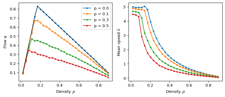
The fundamental diagram is the relation between traffic density and traffic flow in the stationary state. It is the main macroscopic observable of a traffic model and the one you compare with road measurements (Nagel and Schreckenberg 1992; chowdhury2000statistical?).
Density, flow and speed
On a ring of \(L\) cells with \(N\) cars:
\[ \rho = \frac{N}{L}, \qquad \bar v = \frac{1}{N}\sum_{n=1}^N v_n, \qquad q = \frac{1}{L}\sum_{n=1}^N v_n = \rho\, \bar v . \]
The flow \(q\) is the number of cars that pass a fixed point per time step, averaged over the ring. In simulations you average \(q\) over time after discarding a burn-in period.
Free flow and congested branches
- Free flow. At low density cars rarely interact. Each car moves at about \(v_{\max} - p\) on average, so \(q \approx \rho\,(v_{\max} - p)\) grows linearly with \(\rho\) (chowdhury2000statistical?).
- Congested branch. At high density the gaps limit the speeds and \(q\) decreases with \(\rho\). At \(\rho = 1\) nothing moves.
- Maximum flow. Between the two branches the flow reaches a maximum, the capacity of the road. Randomization lowers the capacity and moves it to lower density.
For \(p = 0\) the diagram is the exact triangle \(q = \min(\rho\, v_{\max},\ 1 - \rho)\) with its maximum at \(\rho = 1/(v_{\max} + 1)\) (chowdhury2000statistical?).
The simulation for \(p = 0\) lies on the exact triangle, which validates the code. For \(p > 0\) the peak is lower and rounded.
Empirical evidence: jams without bottlenecks
Sugiyama and co-workers asked 22 drivers to drive around a circular track of 230 m, starting from a uniform configuration. A stop-and-go wave formed spontaneously and travelled backwards, with no bottleneck on the track (sugiyama2008traffic?). They interpret the jam as a collective instability of free flow that appears when the density exceeds a critical value.
This is the phenomenon that the randomization step produces in the Nagel-Schreckenberg model: jams on a homogeneous ring, triggered by fluctuations. The experiment does not test the specific rules of the model. It shows that a model of homogeneous traffic on a ring must be able to produce such jams.
Exercise
Use the free-flow approximation \(q \approx \rho (v_{\max} - p)\) and the congested branch \(q \approx 1 - \rho\) of the deterministic model to estimate where the maximum flow occurs for \(v_{\max} = 5\) and \(p = 0.3\). Compare with the figure.
Solution
The two lines cross at \(\rho (v_{\max} - p) = 1 - \rho\), so \(\rho^* = 1/(v_{\max} - p + 1) = 1/5.7 \approx 0.175\) and \(q^* \approx 0.82\). The simulated curve for \(p = 0.3\) peaks near \(\rho \approx 0.1\) with \(q\) below 0.5, so at lower density and much lower flow. Randomization also lowers the congested branch below \(1 - \rho\), because stopped cars restart with a delay. The crossing of the two straight lines is only an upper estimate.
Next
Nagel, Kai, and Michael Schreckenberg. 1992. “A Cellular Automaton Model for Freeway Traffic.” Journal de Physique I 2 (12): 2221–29. https://doi.org/10.1051/jp1:1992277.