Flow and Congestion
Module 6: Explorables and Discrete Models
Once the simulator works, the next step is to extract macroscopic observables. In traffic modelling the most important one is the fundamental diagram, the relationship between density and average flow (Nagel and Schreckenberg 1992). The theory is on the page The Fundamental Diagram.
Core activity
Estimate the fundamental diagram \(q(\rho)\) for two values of p_slow, and validate your code against the exact result for p_slow = 0.
Prediction
Exercise
Sketch \(q(\rho)\) for p_slow = 0 before you run anything. Where is the maximum? How should the curve change for p_slow = 0.3?
Solution
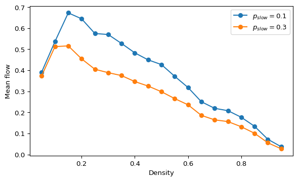
For p_slow = 0 the curve is the triangle \(q = \min(5\rho,\ 1 - \rho)\). It rises with slope \(v_{\max} = 5\), peaks at \(\rho = 1/6 \approx 0.17\) with \(q = 5/6 \approx 0.83\), and falls linearly to \(q = 0\) at \(\rho = 1\). For p_slow = 0.3 the free-flow slope drops to about \(v_{\max} - p = 4.7\), the peak is rounded and much lower, about \(q \approx 0.5\) near \(\rho \approx 0.1\) on a ring of 400 cells, and the congested branch lies below \(1 - \rho\). Compare with the figure on The Fundamental Diagram.
Measure density and flow
Two standard macroscopic quantities are
\[ \rho = \frac{N_{\mathrm{cars}}}{L}, \qquad q(t) = \frac{1}{L}\sum_{i \in \mathrm{cars}} v_i(t). \]
Here \(\rho\) is the density and \(q(t)\) is the instantaneous flow, measured as the mean number of cells traveled per road cell and per time step.
To estimate stationary behavior, average \(q(t)\) after a burn-in window.
Record flow during one run
The simplest extension of the simulator is to track the flow after each update.
def simulate_with_flow(steps, length, density, vmax, p_slow, seed):
    rng = np.random.default_rng(seed)
    occupied, speeds = initialize_road(length=length, density=density, vmax=vmax, rng=rng)

    flow_history = np.zeros(steps)
    flow_history[0] = speeds[occupied].sum() / length

    for t in range(1, steps):
        occupied, speeds = step(
            occupied,
            speeds,
            vmax=vmax,
            p_slow=p_slow,
            rng=rng,
        )
        flow_history[t] = speeds[occupied].sum() / length

    return flow_history
Sweep the density
Now repeat the experiment for many densities.
densities = np.linspace(0.05, 0.95, 19)
mean_flows = []

for density in densities:
    flow_history = simulate_with_flow(
        steps=300,
        length=100,
        density=density,
        vmax=5,
        p_slow=0.3,
        seed=7,
    )
    mean_flows.append(flow_history[100:].mean())
Plotting mean_flows against densities gives the fundamental diagram.
Validation
For p_slow = 0 the stationary flow is \(q = \min(\rho\, v_{\max},\ 1 - \rho)\) (chowdhury2000statistical?). Compare your sweep with this line before you trust the curves for p_slow > 0.
# initialize_road() draws the occupancy at random, so measure the actual density
actual = np.array([
    initialize_road(length=100, density=d, vmax=5, rng=np.random.default_rng(7))[0].mean()
    for d in densities
])
exact = np.minimum(actual * 5, 1 - actual)
sim = np.array([simulate_with_flow(density=d, p_slow=0.0, seed=7)[burn_in:].mean() for d in densities])
print("Largest deviation from the exact p = 0 result:", np.round(np.abs(sim - exact).max(), 3))
Largest deviation from the exact p = 0 result: 0.0Use the measured density \(N/L\), not the target value: on a road of 100 cells the random initialization can differ from the target by several cars.
Compare slowdown probabilities
The most informative parameter to vary is p_slow.
- At small density, cars rarely interact and the flow grows roughly linearly with density.
- At intermediate density, the flow reaches a maximum.
- At high density, braking dominates and the flow drops because congestion limits motion.
Increasing p_slow usually lowers the peak flow and shifts the congested regime earlier.
Practical tip
Use several seeds if you want smoother curves. For example, estimate the mean flow for each density with 5 to 10 trials and then average the stationary values.
Interpretation
- A space-time diagram in a free-flow regime and one in a congested regime show the microscopic picture.
- The flow-density curve shows the macroscopic picture: where the maximum flow occurs and how noise changes it.
Limitations
initialize_road()draws the occupancy at random, so the number of cars fluctuates arounddensity * length. Use the measured density \(N/L\) on the horizontal axis for precise work.- One seed per density gives noisy curves near the maximum.
Next
Nagel, Kai, and Michael Schreckenberg. 1992. “A Cellular Automaton Model for Freeway Traffic.” Journal de Physique I 2 (12): 2221–29. https://doi.org/10.1051/jp1:1992277.