Traffic Extensions
Module 6: Explorables and Discrete Models
The Nagel-Schreckenberg model is a minimal model. This page adds three extensions from the literature and asks one question for each: does it change the fundamental diagram qualitatively, or only shift the numbers? The code is in amlab/cellular_automata/traffic_models.py, which stores only car positions and speeds and runs much faster than the cell-based lab code.
Core activity
Reproduce the slow-to-start experiment below and explain why two initial conditions give two different flows at the same density. The other two extensions are optional.
Prediction
Exercise
Before you run the code, write down for each extension whether you expect a new feature in \(q(\rho)\) (a new branch, a jump, a change of slope) or only a lower or higher curve.
Solution
Slow-to-start adds a new feature: a second, metastable high-flow branch and hysteresis. Slow vehicles on one lane change the slope of the free-flow branch to roughly the speed of the slowest cars. Two lanes with identical cars only give a curve close to the single-lane one, per lane. The table under Interpretation summarizes the results, and the figures below show them.
Slow-to-start rule
In the velocity-dependent randomization (VDR) model, a car that was stopped in the previous step brakes randomly with probability \(p_0\), and a moving car with the usual probability \(p\) (barlovic1998metastable?). With \(p_0 > p\), cars leave a jam more slowly than they drive in free flow. This is one of the slow-to-start rules.
In nasch_step() this is one extra line: build the vector of randomization probabilities from the speeds before acceleration.
prob = np.full(x.size, p)
prob[v == 0] = p0          # stopped cars start with a delay
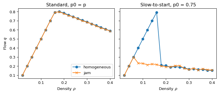
Barlovic et al. show that this rule produces metastable high-flow states and hysteresis in the fundamental diagram (barlovic1998metastable?). To see it, start from two initial conditions at every density: evenly spaced moving cars (homogeneous) and one compact jam.
In the standard model both starts give the same curve. With slow-to-start there is a density range where the homogeneous start keeps a high flow and the jammed start stays at a low flow. The high-flow state is metastable: a large enough perturbation sends it to the jammed branch. This changes the diagram qualitatively: the flow is no longer a function of density alone, it also depends on history.
Slow vehicles
Give a fraction \(f\) of the cars a lower maximum speed \(v_{\max}^{\text{slow}}\). On a single lane nobody can overtake, so at low density every fast car ends up behind a slow one and the cars form platoons (knospe1999disorder?).
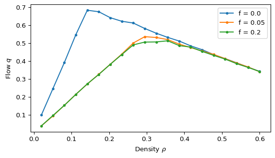
Even a small fraction of slow cars sets the slope of the free-flow branch to roughly \(v_{\max}^{\text{slow}} - p\), the speed of the slowest car. At high density the curves merge, because the gaps limit every car. This also changes the diagram qualitatively at low density.
Optional extension: two lanes
Add a second lane and a symmetric lane-changing rule, as in Rickert et al. (rickert1996two?). In two_lane_step() a car changes lane when its gap ahead is shorter than \(v+1\), the other lane offers a longer gap, the target cell is free, and the gap behind in the other lane is at least \(v_{\max}\). Then each lane applies the Nagel-Schreckenberg rules.
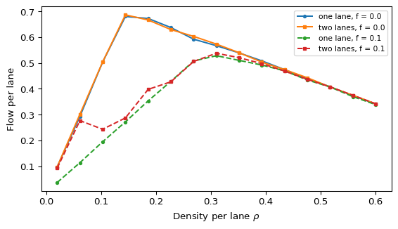
With identical cars, the flow per lane on two lanes stays close to the single-lane curve: a second lane mostly doubles the road, it does not change the shape of the diagram. With slow cars, overtaking is possible, but lane changes need a free gap in the other lane. Knospe et al. found that even a small number of slow cars can still create platoons at low density on two lanes (knospe1999disorder?). In the figure, overtaking restores most of the free flow at the lowest densities, but already at \(\rho \approx 0.1\) the two-lane flow falls towards the one-lane curve with slow cars. Check this with several seeds before you draw conclusions.
Interpretation
| Extension | Qualitative change of \(q(\rho)\)? |
|---|---|
| Slow-to-start (\(p_0 > p\)) | Yes: metastable high-flow branch and hysteresis |
| Fraction of slow vehicles, one lane | Yes: free-flow slope set by the slowest cars, platoons |
| Two lanes, identical cars | No: flow per lane close to the single-lane curve |
Limitations
- Each point is one run with one seed. Near the edges of the hysteresis range, the result depends on the seed and on the run length, because metastable states decay at random times.
- The lane-changing rule here is a simplified symmetric rule. Rickert et al. show that the details of lane changing affect the shape of the diagram (rickert1996two?).
Optional extension: an open road
Exercise
Optional. Replace the ring by an open road of 200 cells: when cell 0 is empty, a car enters there with probability \(\alpha\) per step, and cars that pass the last cell leave. Measure the flow as the number of cars that leave per step, and plot it as a function of \(\alpha\) for \(v_{\max} = 5\) and \(p = 0.3\).
Solution
Store the positions in increasing order, so that the last entry is the front car. The front car sees a free road ahead.
def open_road_flow(alpha, length=200, steps=2000, burn_in=500, vmax=5, p=0.3, seed=0):
    rng = np.random.default_rng(seed)
    x = np.array([], dtype=int)    # positions, increasing
    v = np.array([], dtype=int)
    exits = 0
    for t in range(steps):
        if (x.size == 0 or x[0] > 0) and rng.random() < alpha:
            x = np.concatenate(([0], x))      # a new car enters at cell 0
            v = np.concatenate(([vmax], v))
        gaps = np.append(np.diff(x) - 1, vmax)  # the front car sees a free road
        v = np.minimum(np.minimum(v + 1, vmax), gaps)
        slow = rng.random(x.size) < p
        v = np.where(slow, np.maximum(v - 1, 0), v)
        x = x + v
        out = x >= length                     # cars that pass the last cell leave
        if t >= burn_in:
            exits += out.sum()
        x, v = x[~out], v[~out]
    return exits / (steps - burn_in)


alphas = np.linspace(0.05, 1.0, 12)
fig, ax = plt.subplots(figsize=(6, 3))
ax.plot(alphas, [open_road_flow(a) for a in alphas], marker="o")
ax.set_xlabel(r"Entry probability $\alpha$")
ax.set_ylabel("Cars leaving per step")
plt.tight_layout()
plt.show()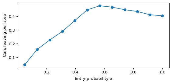
At small \(\alpha\) almost every car that enters also leaves, so the flow is close to \(\alpha\). The flow levels off at about 0.45 near \(\alpha \approx 0.5\) to \(0.7\) and drops slightly, to about 0.40, at \(\alpha = 1\). In that limit a new car enters as soon as cell 0 is free, right behind the previous car, so a dense queue forms near the entrance, and the flow is limited by the rate at which cars leave that queue. Both values stay below the maximum flow of about 0.5 on a ring with the same \(p\). Check the numbers with several seeds.