Budworm: the Model in Code
Module 1: Low-Dimensional Dynamics
Core activity
This page and the next two form the core activity of Session 3: implement the budworm model, integrate it, and wrap it in a Streamlit app.
You will implement the dimensionless budworm model from The Spruce Budworm Model (Strogatz 2024, sec. 3.7):
\[ \frac{dx}{dt} = rx\left(1 - \frac{x}{k}\right) - \frac{x^2}{1 + x^2}. \tag{1}\]
The first term is logistic growth. The second term is predation by birds, with a saturating functional response.
Prediction
Exercise
Before you write code, use Fixed Points and Stability to predict how many positive equilibria you expect for \(r = 0.5\), \(k = 10\), and which ones are stable.
Solution
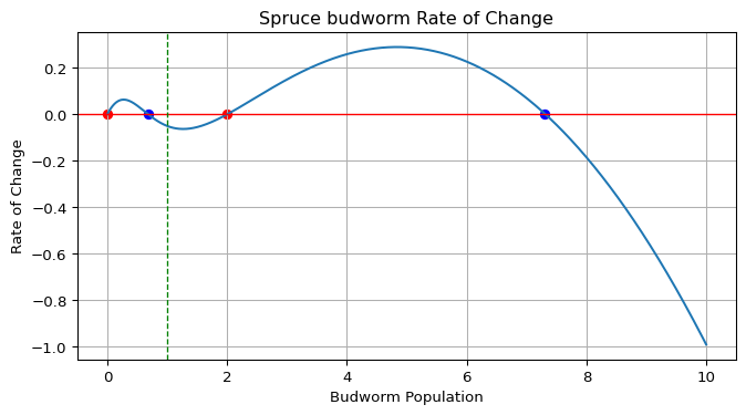
There are three positive equilibria, \(x_a \approx 0.68\), \(x_b = 2\) and \(x_c \approx 7.32\), plus the unstable state \(x = 0\). The slope \(f'(x^*)\) is negative at \(x_a\) and \(x_c\) (stable) and positive at \(x_b\) (unstable). The validation at the end of this page checks these values.
Implementation: the ODE function
Exercise
Create a function that follows the signature required by scipy.integrate.solve_ivp.
- Function name:
spruce_budworm - Parameters:
t(time),x(population),r(growth rate),k(carrying capacity) - Return: the rate of change \(dx/dt\).
- Include a docstring.
def spruce_budworm(t: float, x: float, r: float = 0.5, k: float = 10) -> float:
    """Docstring and type hints"""
    dxdt = # TODO: fill in the equation
    return dxdt
Why do we need t as an input? The equation does not depend on time, but solve_ivp always calls the function as fun(t, y, *args).
Solution
def spruce_budworm(t: float, x: float, r: float = 0.5, k: float = 10) -> float:
    """Dimensionless spruce budworm model (Strogatz, Section 3.7)."""
    return r * x * (1 - x / k) - x**2 / (1 + x**2)
Implementation: the rate plot
This rate plot is the phase portrait of a one-dimensional model: it shows the equilibria and their stability at a glance.
Exercise
Create a function that plots \(dx/dt\) against \(x\) and marks the equilibria.
- Function name:
plot_spruce_budworm_rate - Parameters:
x_t(current population),r,k - Plot \(dx/dt\) for \(x \in [0, k]\) and a horizontal line at zero.
- Mark stable equilibria in blue (where \(dx/dt\) crosses zero from above) and unstable ones in red (from below).
- Mark the current population \(x_t\) with a vertical dashed line.
- Return the figure and axes.
def plot_spruce_budworm_rate(x_t: float, r: float = 0.5, k: float = 10):
    x = np.linspace(0, k, 1000)
    dxdt = # TODO: evaluate the model on the grid
    # TODO: find sign changes of dxdt with np.diff and np.sign
    # TODO: classify each crossing as stable or unstable
    fig, ax = plt.subplots(figsize=(8, 4))
    # TODO: plot the curve, the zero line, the equilibria and x_t
    return fig, ax
Figure 1 shows the expected output.
Hint
- Use
np.linspaceto create the grid of \(x\) values. np.diff(np.sign(dxdt))is nonzero exactly where the sign changes between two grid points.- An equilibrium \(x^*\) is a value where \(dx/dt = 0\). It is stable if small perturbations decay back to \(x^*\), and unstable if they grow.
- A fixed point is stable if \(dx/dt\) decreases as you pass through it. So if
dxdt[i+1] < 0at a crossing, the curve goes from positive to negative and the equilibrium is stable.
Solution
This follows plot_spruce_budworm_rate in amlab/odes_1d/spruce_budworm.py.
def plot_spruce_budworm_rate(x_t: float, r: float = 0.5, k: float = 10):
    """Plot dx/dt against x, mark the equilibria and the current state x_t."""
    x = np.linspace(0, k, 1000)
    dxdt = spruce_budworm(0, x, r, k)

    mask_zerocross = np.diff(np.sign(dxdt)).astype(bool)
    is_stable = np.where(mask_zerocross & (dxdt[1:] < 0))[0]
    is_unstable = np.where(mask_zerocross & (dxdt[1:] > 0))[0]

    fig, ax = plt.subplots(figsize=(8, 4))
    ax.plot(x, dxdt)
    ax.axhline(0, color="red", lw=1)
    ax.scatter(x[is_stable], np.zeros(len(is_stable)), color="blue", zorder=3)
    ax.scatter(x[is_unstable], np.zeros(len(is_unstable)), color="red", zorder=3)
    ax.axvline(x_t, color="green", lw=1, linestyle="--")
    ax.set_xlabel("Budworm population")
    ax.set_ylabel("Rate of change")
    ax.set_title("Spruce budworm rate of change")
    ax.grid()
    return fig, ax
Validation
Compare the crossings found on the grid with the exact roots of the cubic.
import numpy as np

from amlab.odes_1d.budworm_analysis import budworm_equilibria
from amlab.odes_1d.spruce_budworm import spruce_budworm

x = np.linspace(0, 10, 1000)
dxdt = spruce_budworm(0, x, 0.5, 10.0)
grid_roots = x[1:][np.diff(np.sign(dxdt)).astype(bool)]
print("Grid crossings:", np.round(grid_roots, 3))
print("Exact roots:   ", np.round(budworm_equilibria(0.5, 10.0), 3))
Grid crossings: [0.01 0.691 2.002 7.317]
Exact roots: [0.683 2. 7.317]The first crossing is the fixed point \(x = 0\): np.sign(0) is 0, so the step from 0 to a positive value counts as a sign change. The other grid values agree with the exact roots to within the grid spacing \(10/999 \approx 0.01\).
Next
Strogatz, Steven H. 2024. Nonlinear Dynamics and Chaos: With Applications to Physics, Biology, Chemistry, and Engineering. Chapman; Hall/CRC.