Fixed Points and Stability
Module 1: Low-Dimensional Dynamics
A one-dimensional model \(\dot x = f(x)\) is fully described by the graph of \(f\). This page applies that idea to the budworm model \(f(x) = rx(1 - x/k) - x^2/(1+x^2)\) from The Spruce Budworm Model (Strogatz 2024, chap. 2 and Section 3.7).
Fixed points
A fixed point (equilibrium) \(x^*\) satisfies \(f(x^*) = 0\). For the budworm, \(x^* = 0\) is always a fixed point. The others satisfy
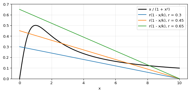
\[ r\left(1 - \frac{x}{k}\right) = \frac{x}{1 + x^2}. \tag{1}\]
The left side is the per capita growth rate, a straight line with intercepts \(r\) and \(k\). The right side is the per capita predation rate. Fixed points are the intersections of the two curves, and there can be one, two or three of them (Strogatz 2024, sec. 3.7; ludwig1978qualitative?).
Linear stability
Write \(x = x^* + \eta\) with \(\eta\) small. A Taylor expansion gives \(\dot\eta \approx f'(x^*)\,\eta\), so the perturbation grows or decays like \(e^{f'(x^*)t}\) (Strogatz 2024, sec. 2.4).
- \(f'(x^*) < 0\): the fixed point is stable.
- \(f'(x^*) > 0\): the fixed point is unstable.
- \(f'(x^*) = 0\): linearization is inconclusive; this happens at a bifurcation.
The time scale of the decay or growth is \(1/|f'(x^*)|\). For the budworm,
\[ f'(x) = r\left(1 - \frac{2x}{k}\right) - \frac{2x}{(1 + x^2)^2}. \]
At \(x^* = 0\), \(f'(0) = r > 0\), so the zero state is always unstable. A small budworm population always grows, because predation vanishes faster than growth as \(x \to 0\) (ludwig1978qualitative?).
The phase line
You can read stability directly from the sign of \(f\): the flow moves right where \(f > 0\) and left where \(f < 0\). Figure 2 shows the rate for \(r = 0.5\) and \(k = 10\).
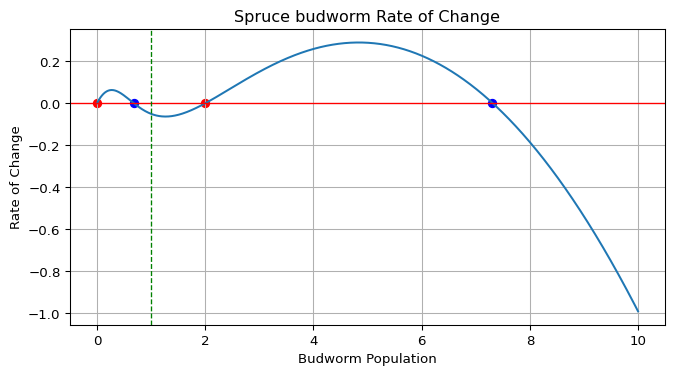
The positive fixed points for these values can be computed exactly, since Equation 1 is a cubic in \(x\).
from amlab.odes_1d.budworm_analysis import budworm_equilibria, budworm_slope

x_star = budworm_equilibria(r=0.5, k=10.0)
for x in x_star:
    s = budworm_slope(x, 0.5, 10.0)
    print(f"x* = {x:.3f}, f'(x*) = {s:+.3f}, {'stable' if s < 0 else 'unstable'}")
x* = 0.683, f'(x*) = -0.203, stable
x* = 2.000, f'(x*) = +0.140, unstable
x* = 7.317, f'(x*) = -0.237, stable
Exercise
Show that the middle fixed point for \(r = 0.5\), \(k = 10\) is exactly \(x^* = 2\).
Solution
Substitute \(x = 2\) in Equation 1: the left side is \(0.5(1 - 0.2) = 0.4\) and the right side is \(2/5 = 0.4\). The other roots of the cubic \(-(r/k)x^3 + rx^2 - (1 + r/k)x + r = 0\) are \(4 \pm \sqrt{11} \approx 0.683\) and \(7.317\).
Next
Strogatz, Steven H. 2024. Nonlinear Dynamics and Chaos: With Applications to Physics, Biology, Chemistry, and Engineering. Chapman; Hall/CRC.