Vicsek Lab: Order Parameter
Module 2: Synchronization and Collective Behaviour
Implementation: the order parameter
The order parameter \(\varphi\) (called \(v_a\) in The Vicsek Model) is defined as the magnitude of the average velocity vector normalized by the speed:
\[ \varphi(t) = \frac{1}{N v_0} \left|\sum_{i=1}^N v_0 \begin{bmatrix} \cos(\theta_i(t)) \\ \sin(\theta_i(t)) \end{bmatrix}\right| = \frac{1}{N} \left|\sum_{i=1}^N \begin{bmatrix} \cos(\theta_i(t)) \\ \sin(\theta_i(t)) \end{bmatrix}\right|. \tag{1}\]
You can compute this at each time step to see how the system evolves. In the disordered phase, \(\varphi \approx 0\) because the headings are random and cancel out. In the ordered phase, \(\varphi \approx 1\) because all particles align in the same direction.
Exercise
Implement Equation 1.
def vicsek_order_parameter(theta: np.ndarray, v0: float = 0.03) -> float:
    # TODO: Compute the order parameter phi based on the headings theta
    return phi
Solution
The speed \(v_0\) cancels, so np.abs(np.mean(np.exp(1j * theta))) gives the same value.
def vicsek_order_parameter(theta: np.ndarray, v0: float = 0.03) -> float:
    """
    Compute the normalized order parameter (mean velocity divided by v0), as in Vicsek et al. (1995).
    """
    vx = v0 * np.cos(theta)
    vy = v0 * np.sin(theta)
    avg_vx = np.mean(vx)
    avg_vy = np.mean(vy)
    return float(np.sqrt(avg_vx**2 + avg_vy**2) / v0)
Experiment: reproduce Figure 2
Try to reproduce Figure 2 of the original paper (Vicsek et al. 1995), which shows the order parameter \(\varphi\) as a function of noise \(\eta\) and of the density \(\rho = N / L^2\). Run simulations for different values of \(N\), \(L\), and \(\eta\), compute the order parameter at each time step, and then average it over time to get a single value for each combination of parameters.
For reference, here are the parameters used in the original paper for Figure 2(a):
- Number of particles \(N\): from 40 up to 10000. Start with the two smallest values, 40 and 100, and try larger ones only if you have time.
- Density \(\rho\): constant at 4.0
- Box size L: computed from density and number of particles, so \(L = \sqrt{N / \rho}\).
- Noise \(\eta\): try several values between 0.0 and 5.0
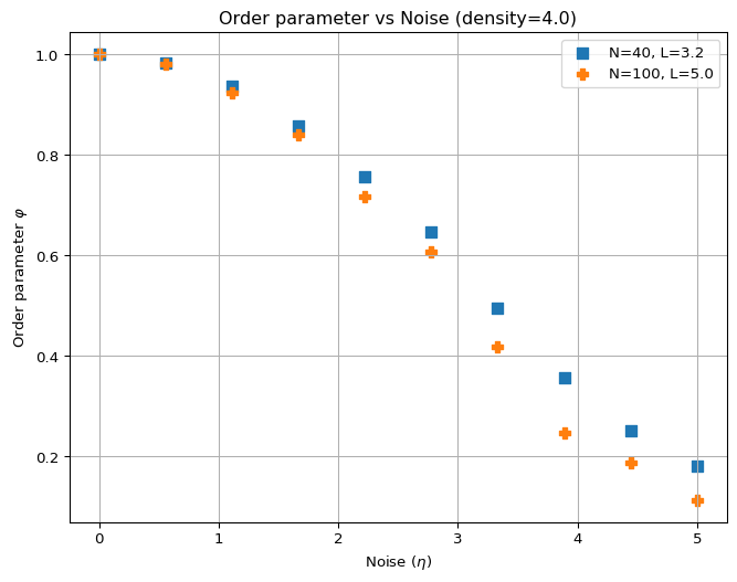
Figure 1 shows the order parameter as a function of noise for different values of \(N\) at a constant density of \(\rho = 4.0\). This is a small sample of the figure you want to produce. You should see that as noise increases, the order parameter decreases, indicating a transition from an ordered phase to a disordered phase. The larger the number of particles, the sharper this transition should be.
And here are the parameters for Figure 2(b):
- Density \(\rho\): try several values between 0.1 and 10.0. Higher values will take longer to compute, so start with a few values like 0.1, 1.0, and 4.0. In addition, you can distribute the values logarithmically so that you have more points at low densities where they compute faster.
- Box size \(L\): constant at 20.
- Number of particles \(N\): computed from density and box size, so \(N = \rho L^2\).
- Noise \(\eta\): constant. The course uses \(\eta = 2.0\); check the value in the caption of Figure 2(b) of Vicsek et al. (1995).
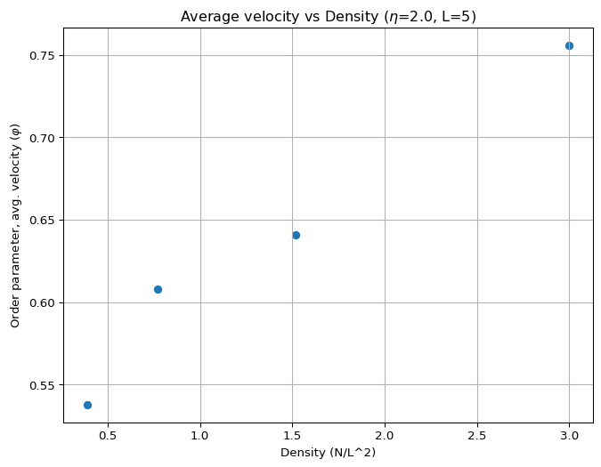
Figure 2 shows the order parameter as a function of density for different values of \(N\) at a constant noise level. This is a small sample of the figure you want to generate. At low densities the order parameter is small (disordered phase), and at high densities it grows toward one (ordered phase). In a small box it does not reach zero at low density, because few particles give a large noise floor of order \(1/\sqrt{N}\).
Exercise
Write a function that runs the model and returns the time-averaged order parameter. Use it to draw your versions of Figure 1 and Figure 2 with the parameters above.
def time_averaged_order(num_boids, box_size, noise, steps=5000, avg_steps=1000):
    xy, theta = initialize_particles(num_boids, box_size)
    ls_phi = []
    for step in range(steps):
        # TODO: advance one step with vicsek_equations

        # TODO: in the last avg_steps steps, store the order parameter
        pass
    # TODO: return the mean of the stored values
Hint
Start short. With steps=1000 and avg_steps=200 each run of \(N = 100\) takes well under a second with the vectorized update. Increase the number of steps once the curves look right, and check that the result does not change much.
Solution
import numpy as np
import matplotlib.pyplot as plt


def time_averaged_order(num_boids, box_size, noise, steps=5000, avg_steps=1000):
    xy, theta = initialize_particles(num_boids, box_size)
    ls_phi = []
    for step in range(steps):
        xy, theta = vicsek_equations(xy, theta, noise=noise, box_size=box_size)
        if step >= steps - avg_steps:
            ls_phi.append(vicsek_order_parameter(theta))
    return np.mean(ls_phi)


# Figure 2(a): phi against noise at fixed density
density = 4.0
noises = np.linspace(0.0, 5.0, 10)
for num_boids in [40, 100]:
    box_size = np.sqrt(num_boids / density)
    phi = [time_averaged_order(num_boids, box_size, eta) for eta in noises]
    plt.plot(noises, phi, "o", label=f"N = {num_boids}")
plt.xlabel(r"Noise $\eta$")
plt.ylabel(r"Order parameter $\varphi$")
plt.legend()
plt.show()

# Figure 2(b): phi against density at fixed noise and box size
box_size = 20
densities = np.logspace(-1, np.log10(4.0), 6)
phi = [
    time_averaged_order(int(rho * box_size**2), box_size, noise=2.0)
    for rho in densities
]
plt.plot(densities, phi, "o")
plt.xlabel(r"Density $\rho$")
plt.ylabel(r"Order parameter $\varphi$")
plt.show()
The second part is slow for \(\rho = 4\) (\(N = 1600\)). Lower the number of steps, or use a smaller box as in Figure 2, while you test your code.
Interpretation
- Both figures show the two routes to order in Vicsek et al. (1995): less noise, or more density.
- The curves for \(N = 40\) and \(N = 100\) are close. With systems this small you cannot tell whether the transition is continuous or discontinuous; that question needed much larger simulations (gregoire2004onset?; chate2008collective?).
References
Vicsek, Tamás, András Czirók, Eshel Ben-Jacob, Inon Cohen, and Ofer Shochet. 1995. “Novel Type of Phase Transition in a System of Self-Driven Particles.” Physical Review Letters 75 (6): 1226.