Special Rules and Theorems
Module 6: Explorables and Discrete Models
A few elementary rules and a few theorems appear again and again in the cellular automata literature. This page collects them briefly.
Rule 90 and Pascal’s triangle
Rule 90 sets each cell to the sum of its two neighbours modulo 2,
\[ x_i^{t+1} = \big(x_{i-1}^t + x_{i+1}^t\big) \bmod 2 . \]
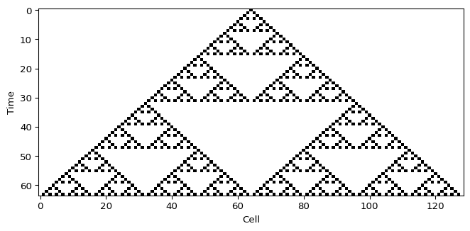
The rule is additive: the evolution of the sum (mod 2) of two initial rows is the sum of their evolutions (Wolfram 1983). Started from a single seed at cell 0, the state at time \(t\) and position \(i = 2k - t\) is \(\binom{t}{k} \bmod 2\), the rows of Pascal’s triangle modulo 2. The pattern is self-similar, with fractal dimension \(\log_2 3 \approx 1.585\) (Wolfram 1983).
The assert in the code checks the Pascal identity for every cell of the figure.
Rule 110 is universal
Rule 110 belongs to class 4. Cook proved that it can emulate a cyclic tag system, and therefore any Turing machine. This settled a conjecture of Wolfram (cook2004universality?). The proof needs an infinite lattice with a periodic background pattern and specific localized structures on it.
A consequence is that some questions about the long-run behaviour of Rule 110, such as whether a given pattern ever appears, are undecidable in general.
Langton’s lambda
Pick one state as quiescent, here 0. Langton’s parameter \(\lambda\) is the fraction of neighbourhood configurations that the rule maps to a non-quiescent state (langton1990computation?). For an elementary rule, \(\lambda\) is the number of 1s in the rule table divided by 8.
Langton studied larger rule spaces (more states and larger neighbourhoods). As \(\lambda\) increases from 0, typical rules move from fixed-point behaviour, through periodic behaviour, to chaotic behaviour, and the complex rules concentrate near the transition between ordered and chaotic regimes (langton1990computation?). With only 256 rules and 9 possible values of \(\lambda\), the elementary rules are too few to show this cleanly. The output below shows that rules 108 (class 2), 30 and 90 (class 3) all have \(\lambda = 1/2\).
from amlab.cellular_automata.elementary import langton_lambda

for rule in (32, 108, 30, 90, 110):
    print(f"Rule {rule:3d}: lambda = {langton_lambda(rule):.3f}")
Rule 32: lambda = 0.125
Rule 108: lambda = 0.500
Rule 30: lambda = 0.500
Rule 90: lambda = 0.500
Rule 110: lambda = 0.625Garden-of-Eden configurations
A Garden-of-Eden configuration has no predecessor: no configuration evolves into it in one step. Such configurations can only appear as initial conditions.
Two configurations are mutually erasable if they differ on a finite set of cells and have the same successor. Moore showed that a cellular automaton with mutually erasable configurations has Garden-of-Eden configurations (moore1962machine?). Myhill proved the converse (myhill1963converse?). Together:
Garden-of-Eden theorem. A cellular automaton on \(\mathbb{Z}^d\) has a Garden-of-Eden configuration if and only if it has two mutually erasable configurations.
In other words, the global map is surjective exactly when it is injective on configurations that differ in finitely many cells.
Exercise
Find two configurations of a ring of \(N = 4\) cells that Rule 184 maps to the same successor. Explain why this implies that some configurations of the ring have no predecessor.
Solution
import itertools
import numpy as np
from amlab.cellular_automata.elementary import step_eca

successors = {}
for bits in itertools.product((0, 1), repeat=4):
    key = "".join(map(str, step_eca(np.array(bits), 184)))
    successors.setdefault(key, []).append("".join(map(str, bits)))
for image, preimages in successors.items():
    if len(preimages) > 1:
        print(image, "<-", preimages)
1010 <- ['0011', '0101', '1100']
0101 <- ['0110', '1001', '1010']For example 1100 and 0101 both map to 1010 on a ring of 4 cells. A map from the finite set of \(2^N\) configurations to itself that is not injective is not surjective either, so some configurations on the ring have no predecessor.
Next
Wolfram, Stephen. 1983. “Statistical Mechanics of Cellular Automata.” Reviews of Modern Physics 55 (3): 601–44. https://doi.org/10.1103/RevModPhys.55.601.