matplotlib.pyplot.
Module 1: Low-Dimensional Dynamics
This page continues CDIMA: Phase Plane. You add the nullclines and the fixed point to the phase plane (Strogatz 2024, sec. 6.1 and 8.3).
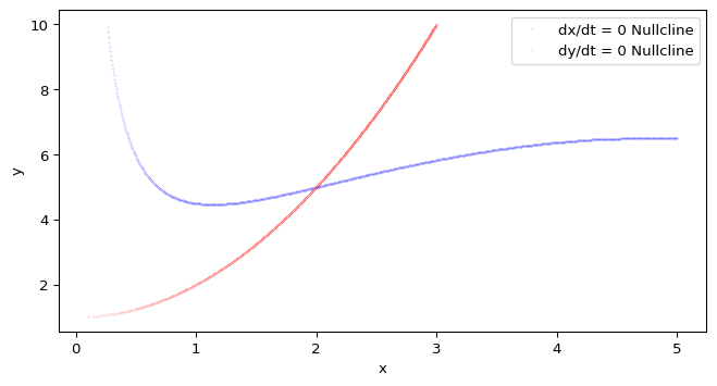
Solve \(\dot y = 0\) by hand for \(x > 0\). You should get \(y = 1 + x^2\). Where do you expect it to cross the \(x\)-nullcline for \(a = 10\)?
From \(\dot x = 0\): \(y = (a - x)(1 + x^2)/(4x)\). From \(\dot y = 0\) with \(x > 0\): \(y = 1 + x^2\). Setting them equal gives \(a - x = 4x\), so \(x^* = a/5\). For \(a = 10\) the crossing is at \((2, 5)\).
In addition to trajectories, we can also plot nullclines in the phase plane. Nullclines are curves where the derivative of one of the variables is zero. They help us identify equilibrium points and understand the flow of trajectories.
matplotlib.pyplot.
How can we find the nullclines for the CDIMA system? We have two options:
The intersection points of the nullclines correspond to equilibrium points of the system.
Pick one of these methods to compute the nullclines for the CDIMA system with \(a = 10\), \(b = 4\), and plot them in the phase plane as in Figure 1.
# Define the limits for the grid
x_min, x_max = 0.1, 5
y_min, y_max = 0, 10
num_points = 1000  # Number of points in the grid

# Create a grid of points
x_values = np.linspace(x_min, x_max, num_points)
y_values = np.linspace(y_min, y_max, num_points)
x_grid, y_grid = np.meshgrid(x_values, y_values)
# meshgrid creates two 2D arrays:
# x_grid and y_grid, where each element (i,j) corresponds to the
# coordinates (x_values[i], y_values[j]) in the phase plane.

# Evaluate the derivatives at each point
dx_dt: np.ndarray
dy_dt: np.ndarray
dx_dt, dy_dt = cdima(0, [x_grid, y_grid], a, b)

# Extract nullcline data:
# Find where dx_dt changes sign (zero crossings)
dxdt_zero_crossings = np.where(np.diff(np.sign(dx_dt), axis=0))
dxdt_nullcline_x = x_grid[dxdt_zero_crossings]
dxdt_nullcline_y = y_grid[dxdt_zero_crossings]

# Extract nullcline data - Find where dy_dt changes sign (zero crossings)
dydt_zero_crossings = np.where(np.diff(np.sign(dy_dt), axis=1))
dydt_nullcline_x = x_grid[dydt_zero_crossings]
dydt_nullcline_y = y_grid[dydt_zero_crossings]
Now you can plot the nullclines using matplotlib Recommendation: do not join the points! There is no guarantee that the sequence of points in dxdt_nullcline_x and dxdt_nullcline_y (or dydt_nullcline_x and dydt_nullcline_y) will form a continuous curve, so it’s better to plot them as individual points (e.g., using 'o' markers) rather than trying to connect them with lines.
With the arrays from the hint, plot each nullcline as a cloud of points. The analytical curves from the Prediction exercise should lie on top of them.
fig, ax = plt.subplots(figsize=(8, 4))
ax.plot(dxdt_nullcline_x, dxdt_nullcline_y, "o", ms=0.5, color="blue", label="dx/dt = 0")
ax.plot(dydt_nullcline_x, dydt_nullcline_y, "o", ms=0.5, color="red", label="dy/dt = 0")
x_line = np.linspace(0.1, 5, 200)
ax.plot(x_line, (a - x_line) * (1 + x_line**2) / (4 * x_line), "k--", lw=0.8, label="analytical")
ax.plot(x_line, 1 + x_line**2, "k--", lw=0.8)
ax.set_xlim(0, 5)
ax.set_ylim(0, 10)
ax.set_xlabel("x")
ax.set_ylabel("y")
ax.legend()
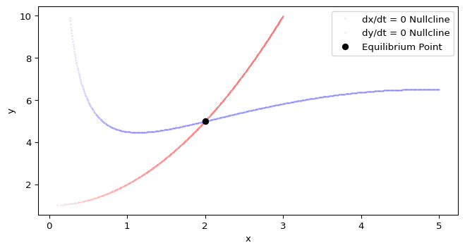
plt.show()The intersection points of the nullclines correspond to equilibrium points (equilibria) of the system. In other words, they are points where both \(\dot x = 0\) and \(\dot y = 0\) simultaneously.
To find the equilibrium points, we can look for the coordinates where the x-nullcline and y-nullcline intersect. This can be done by checking for points that are close to each other in both nullcline datasets or by using a more systematic approach (e.g., clustering or root-finding methods).
In Python, we can use the scipy.optimize.fsolve() function to find the roots of the system of equations defined by the nullclines. This will give us the coordinates of the equilibrium points.
from scipy.optimize import fsolve

a, b = 10, 4

# We need to define a function that represents the system of
# equations for the nullclines
def cdima_fixed(xy: np.ndarray) -> np.ndarray:
    return cdima(None, xy, a, b)

equilibrium_point = fsolve(cdima_fixed, [1, 1])  # Initial guess for the equilibrium point
print(f"Equilibrium point: x={equilibrium_point[0]:.2f}, y={equilibrium_point[1]:.2f}")
If we have done things well, plotting the equilibrium point on the phase plane should show that it lies at the intersection of the nullclines.
scipy.optimize.fsolve() and matplotlib.pyplot.
The analytical fixed point is \((a/5, 1 + (a/5)^2) = (2, 5)\) for \(a = 10\). Check that fsolve returns it and that the analytical nullclines pass through it.
print(f"fsolve: ({equilibrium_point[0]:.4f}, {equilibrium_point[1]:.4f}), exact: (2, 5)")
x_test = 2.0
print("x-nullcline at x = 2:", (a - x_test) * (1 + x_test**2) / (4 * x_test))
print("y-nullcline at x = 2:", 1 + x_test**2)
fsolve: (2.0000, 5.0000), exact: (2, 5)
x-nullcline at x = 2: 5.0
y-nullcline at x = 2: 5.0