Excitability
Module 1: Low-Dimensional Dynamics
Reading
- Compulsory: Strogatz (2024), Section 7.5 on relaxation oscillators.
- Recommended: (ellner2006dynamic?), chapter on neural and excitable dynamics.
A system is excitable if it has a stable rest state, small perturbations decay back to rest, and perturbations above a threshold produce a large excursion before the system returns to rest. Nerve cells behave this way: a small current injection changes the membrane potential slightly, while a larger one triggers an action potential (hodgkin1952quantitative?; Strogatz 2024).
Background: the Hodgkin-Huxley model
Hodgkin and Huxley described the membrane potential \(V\) of the squid giant axon with four ODEs: one for \(V\) and three for gating variables \(m\), \(h\), \(n\) that control the sodium and potassium conductances (hodgkin1952quantitative?):
\[ C\dot V = I - \bar g_{\text{Na}} m^3 h (V - V_{\text{Na}}) - \bar g_{\text{K}} n^4 (V - V_{\text{K}}) - g_L (V - V_L), \]
with each gating variable relaxing to a voltage-dependent steady state. The model reproduced the shape and speed of the action potential measured in experiments. Hodgkin and Huxley shared the 1963 Nobel Prize in Physiology or Medicine with John Eccles, for discoveries on the ionic mechanisms of excitation and inhibition in nerve cell membranes.
Four variables are hard to analyse geometrically. The two-variable models of this session keep the essential structure and can be studied in the phase plane (FitzHugh 1961; morris1981voltage?).
The ingredients
- A fast variable (membrane potential) with an S-shaped, or cubic, nullcline. The middle branch has positive feedback: a small depolarization opens channels that depolarize further.
- A slow recovery variable that eventually pulls the fast variable back.
- A separation of time scales: the fast variable changes much faster than the slow one, so trajectories jump quickly between the outer branches of the cubic nullcline and drift slowly along them (Strogatz 2024, sec. 7.5).
The threshold is not a sharp number in general. In FitzHugh’s analysis it is a narrow band in the phase plane near the middle branch of the cubic nullcline (“quasi-threshold”) (FitzHugh 1961).
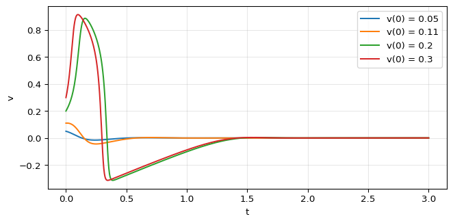
The response is all or nothing: the spikes started from \(v(0) = 0.2\) and \(0.3\) have almost the same height, far above the size of the kick.
Exercise
In Figure 1 the rest state is \((v, w) = (0, 0)\). Use the Jacobian to show that it is stable.
Solution
With \(f(v) = v(1-v)(v - \alpha)\), \(f'(0) = -\alpha\). The Jacobian at the origin is \(\begin{pmatrix} -\alpha/\epsilon & -1/\epsilon \\ 1 & -\gamma \end{pmatrix} = \begin{pmatrix} -10 & -100 \\ 1 & -0.5 \end{pmatrix}\), with \(\tau = -10.5 < 0\) and \(\Delta = 5 + 100 > 0\). The origin is stable. Excitability is a global property: it cannot be seen in the linearization.
Next
FitzHugh, Richard. 1961. “Impulses and Physiological States in Theoretical Models of Nerve Membrane.” Biophysical Journal 1 (6): 445–66. https://doi.org/10.1016/S0006-3495(61)86902-6.
Strogatz, Steven H. 2024. Nonlinear Dynamics and Chaos: With Applications to Physics, Biology, Chemistry, and Engineering. Chapman; Hall/CRC.