Morris-Lecar Model
Module 1: Low-Dimensional Dynamics
Morris and Lecar built a model of the voltage oscillations of the barnacle giant muscle fiber, with two non-inactivating conductances: an excitatory calcium current and a potassium recovery current (morris1981voltage?). Unlike FitzHugh-Nagumo, every term has a physiological meaning.
The equations
With membrane potential \(V\) and the fraction \(n\) of open potassium channels,
\[ \begin{aligned} C\dot V &= I_{\text{app}} - g_{\text{Ca}}\, m_\infty(V)(V - V_{\text{Ca}}) - g_{\text{K}}\, n\,(V - V_{\text{K}}) - g_L (V - V_L),\\ \dot n &= \phi\,\frac{n_\infty(V) - n}{\tau_n(V)}, \end{aligned} \tag{1}\]
\[ m_\infty(V) = \tfrac12\left[1 + \tanh\frac{V - V_1}{V_2}\right],\quad n_\infty(V) = \tfrac12\left[1 + \tanh\frac{V - V_3}{V_4}\right],\quad \tau_n(V) = \operatorname{sech}\frac{V - V_3}{2V_4}. \]
The calcium activation \(m\) is assumed instantaneous, \(m = m_\infty(V)\), which reduces the model to two variables (morris1981voltage?). This is the form given by Lecar in Scholarpedia, with the rate constant written as \(\phi\).
amlab/odes_2d/morris_lecar.py implements Equation 1 with default values \(C = 20\), \(g_{\text{Ca}} = 4\), \(g_{\text{K}} = 8\), \(g_L = 2\) (conductances in mS/cm², capacitance in µF/cm²), \(V_{\text{Ca}} = 120\), \(V_{\text{K}} = -84\), \(V_L = -60\), \(V_1 = -1.2\), \(V_2 = 18\), \(V_3 = 2\), \(V_4 = 30\) (all in mV) and \(\phi = 0.04\). The results below are for these values.
What the simulations show
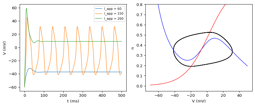
With these parameters:
- for small currents (\(I_{\text{app}} = 60\)) the model rests at a stable fixed point;
- for intermediate currents (\(I_{\text{app}} = 150\)) it fires periodically;
- for large currents (\(I_{\text{app}} = 260\)) the membrane stays depolarized at a new stable fixed point.
The rest state loses stability through a pair of complex eigenvalues, a Hopf bifurcation. You can locate it with the numerical Jacobian of CDIMA: Stability and the Hopf Point:
from scipy.optimize import brentq, fsolve


def max_real_eigenvalue(i_app, h=1e-6):
    fp = fsolve(lambda y: morris_lecar(0, y, i_app), [-30.0, 0.1])
    jac = np.zeros((2, 2))
    for j in range(2):
        e = np.zeros(2)
        e[j] = h
        jac[:, j] = (morris_lecar(0, fp + e, i_app) - morris_lecar(0, fp - e, i_app)) / (2 * h)
    return np.linalg.eigvals(jac).real.max()


print(f"Lower Hopf point: I_app = {brentq(max_real_eigenvalue, 90, 110):.1f}")
print(f"Upper Hopf point: I_app = {brentq(max_real_eigenvalue, 220, 240):.1f}")
Lower Hopf point: I_app = 101.8
Upper Hopf point: I_app = 235.1Simulations started far from rest already oscillate for \(I_{\text{app}} \approx 96\), below the lower Hopf point near 101.8. In that range a stable rest state and a stable limit cycle coexist, which indicates a subcritical Hopf bifurcation for this parameter set. Other parameter sets make the Morris-Lecar model start firing through a saddle-node bifurcation instead, at arbitrarily low frequency; this is why it is used to compare different classes of neural excitability (ellner2006dynamic?).
Exercise
Derive the \(V\)-nullcline shown in Figure 1 from Equation 1.
Solution
Set \(\dot V = 0\) and solve for \(n\): \(n = \dfrac{I_{\text{app}} - g_{\text{Ca}} m_\infty(V)(V - V_{\text{Ca}}) - g_L(V - V_L)}{g_{\text{K}}(V - V_{\text{K}})}\). The \(n\)-nullcline is \(n = n_\infty(V)\).
Optional extension
Run python amlab/odes_2d/morris_lecar.py for the interactive version, then find the smallest current at which the model fires when you start from the rest state and when you start from \(V = 20\) mV.