Cascade Simulation

Module 5: Complex Networks

In this lab you implement the Motter-Lai model, check it on cases you can solve by hand, and measure how the cascade size depends on the tolerance \(\alpha\) and on the trigger. The reference implementation lives in amlab/networks_cascades/.

Core activity

Implement the cascade, validate it, and produce the plot of \(G\) against \(\alpha\) for random and load-based triggers on a Barabási-Albert and an Erdős-Rényi graph.

Prediction

Go back to the two questions at the end of The Iberian Blackout. Write your answers down before you run any code.

Implementation

Complete the two functions below. Use nx.betweenness_centrality(G, normalized=False) for the load.

import networkx as nx


def node_loads(G):
    """Return a dict node -> number of shortest paths through the node."""
    # TODO
    return loads


def run_cascade(G, trigger, alpha):
    """Remove trigger, then remove overloaded nodes until none is left.

    Returns G_ratio = (largest component after the cascade) / N.
    """
    loads0 = node_loads(G)
    capacity = # TODO: (1 + alpha) * initial load, for every node
    H = G.copy()
    H.remove_node(trigger)
    while True:
        loads = # TODO: loads on the damaged network H
        overloaded = # TODO: list of nodes with load > capacity
        if not overloaded:
            break
        # TODO: remove the overloaded nodes from H
    return # TODO

Solved: node_loads() and run_cascade()

def node_loads(G):
    return nx.betweenness_centrality(G, normalized=False)


def run_cascade(G, trigger, alpha, tol=1e-9):
    loads0 = node_loads(G)
    capacity = {v: (1 + alpha) * load for v, load in loads0.items()}
    H = G.copy()
    H.remove_node(trigger)
    while True:
        loads = node_loads(H)
        overloaded = [v for v, load in loads.items() if load > capacity[v] + tol]
        if not overloaded:
            break
        H.remove_nodes_from(overloaded)
    largest = max(nx.connected_components(H), key=len) if len(H) else set()
    return len(largest) / G.number_of_nodes()

The small tolerance tol protects the test load > capacity from rounding errors: with \(\alpha = 0\) an unchanged load must not count as an overload.

Validation

Check your code on cases with a known answer before you trust any plot. The chunk below uses the amlab version; run the same checks on yours.

import networkx as nx
import numpy as np

from amlab.networks_cascades import run_cascade, select_trigger, cascade_curve

# A cycle has equal loads everywhere. Removing one node turns it into a path.
C = nx.cycle_graph(12)
print("cycle, alpha = 10:", run_cascade(C, 0, alpha=10).G_ratio, "expected", 11 / 12)

# The centre of a star carries every shortest path.
S = nx.star_graph(10)
print("star, centre removed:", run_cascade(S, 0, alpha=1).G_ratio, "expected", 1 / 11)

# Very large alpha: only the trigger is lost on a well-connected graph.
G = nx.barabasi_albert_graph(100, 3, seed=1)
r = run_cascade(G, select_trigger(G, "load"), alpha=100)
print("BA, alpha = 100: failed per step", r.failed_per_step)

cycle, alpha = 10: 0.9166666666666666 expected 0.9166666666666666
star, centre removed: 0.09090909090909091 expected 0.09090909090909091
BA, alpha = 100: failed per step [1]

Exercise

Explain the output for the cycle with \(\alpha = 10\). Then predict what happens on the same cycle with \(\alpha = 0\) and check it.

Solution

After the removal the cycle becomes a path of 11 nodes. Loads grow near the middle of the path, but with \(\alpha = 10\) no node exceeds its capacity, so \(G = 11/12\). With \(\alpha = 0\) the nodes near the middle of the path carry more shortest paths than before, so they fail and the cascade cuts the path into pieces. Run run_cascade(C, 0, alpha=0) to see the final value.

Experiment

Now sweep \(\alpha\). For random triggers, average over several trials. The graphs have \(N = 150\) nodes and the same number of edges, so the executed chunk stays fast.

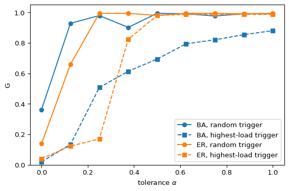
Figure 1: Relative size G of the largest component after a Motter-Lai cascade, as a function of the tolerance alpha. Barabási-Albert (BA) and Erdős-Rényi (ER) graphs with N = 150 and the same number of edges. Random triggers are averaged over 5 trials.

Interpretation

Compare Figure 1 with your predictions:

• For which graph and which trigger does the cascade stay small at small \(\alpha\)?
• How large must \(\alpha\) be before the highest-load trigger stops causing a large cascade on the BA graph?
• Motter and Lai found that heterogeneous networks are fragile to load-based attacks (motter2002cascade?). Does your plot agree? With a single graph realization of 150 nodes, which features of the curves would you trust and which not?

Limitations

• Load follows shortest paths. Electric power follows Kirchhoff’s laws and spreads over all parallel paths.
• The model has no time: the redistribution is instantaneous. (schafer2018dynamically?) show that transient dynamics of a few seconds matter for real grid cascades.
• Every node has the same relative margin \(\alpha\). Real equipment has heterogeneous limits and protection settings.
• A node fails deterministically as soon as \(L_i > C_i\).
• A single BA graph with \(N = 150\) gives noisy curves. Average over several graphs before you draw conclusions.

Optional extension

• Average the curves over 10 graph realizations and add error bars.
• Replace the trigger “highest load” with “highest degree” (select_trigger(G, "degree")). Do the two rankings give the same cascade?
• Load a real network from data/ (for example the USA flights graph) and repeat the sweep on its largest component. Use nx.betweenness_centrality(G, k=..., seed=...) if the exact computation is too slow.

Swing Equation