Drawing Graphs

Module 5: Complex Networks

Toolkit page

This page is self-study material for Session 23. It continues Edges and Weights.

This page draws graphs with networkx and Matplotlib. The first chunk rebuilds the country graph from the previous page.

import matplotlib.pyplot as plt
import networkx as nx

G = nx.Graph()
G.add_node("Spain", population=47_000_000)
G.add_node("Portugal", population=10_000_000)
G.add_node("France", population=67_000_000)
G.add_node("Italy", population=60_000_000)
G.add_edge("Spain", "Portugal", distance=600)
G.add_edge("Spain", "France", distance=1000)
G.add_edge("France", "Italy", distance=800)
G.add_edge("USA", "Canada", distance=3000)
G.add_edge("Netherlands", "Germany", distance=500)
G.add_edge("Germany", "France", distance=900)
G.nodes["USA"]["population"] = 331_000_000
G.nodes["Canada"]["population"] = 38_000_000
G.nodes["Netherlands"]["population"] = 17_000_000
G.nodes["Germany"]["population"] = 83_000_000

Visualization

Printing the graph object gives you a summary of its structure, but it does not show the connections. To visualize the graph, you can use the draw() function from networkx, which uses Matplotlib to display the graph.

# Draw the graph
nx.draw(
    G,
    with_labels=True,  # show node labels (IDs)
    node_color='lightblue',  # color of the nodes (vertices)
    edge_color='gray',  # color of the edges (links)
    node_size=2000,  # size of the nodes (vertices)
    font_size=12  # size of the labels (IDs)
    )
plt.show()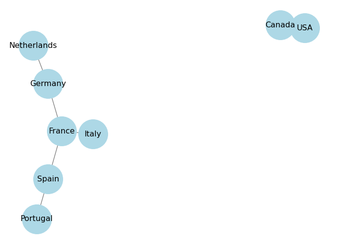

Layouts

The draw() function has a pos parameter that lets you specify the layout of the graph. A layout is a way to position the nodes in the graph for visualization. networkx provides several built-in layouts, such as spring_layout, circular_layout and shell_layout.

Circular layout arranges the nodes in a circle. You can control the distance between the nodes using the scale parameter, higher values will make the nodes farther apart.

# Use the circular layout for visualization
pos = nx.circular_layout(G, scale=2)  # scale controls the distance between the nodes
nx.draw(
    G,
    pos=pos,  # specify the layout
    with_labels=True,
    node_color='lightblue',
    edge_color='gray',
    node_size=2000,
    font_size=12
    )
plt.show()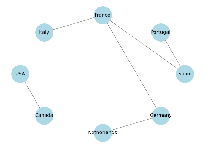

Spring layout uses a force-directed algorithm to position the nodes in a way that minimizes edge crossings and evenly distributes the nodes. You can control the distance between the nodes using the k parameter, which is a scaling factor for the optimal distance between nodes. Higher values will make the nodes farther apart. You can also control the number of iterations of the algorithm using the iterations parameter.

# Use the spring layout for visualization
pos = nx.spring_layout(G, k=0.5, iterations=20)
nx.draw(
    G,
    pos=pos,  # specify the layout
    with_labels=True,
    node_color='lightblue',
    edge_color='gray',
    node_size=2000,
    font_size=12
    )
plt.show()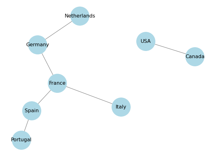

Shell layout arranges the nodes in concentric circles. You can specify which nodes belong to which circle using the nlist parameter, which is a list of lists of nodes.

nlist = [["Spain", "Portugal", "France", "Italy"], ["Netherlands", "Germany", "USA", "Canada"]]
pos = nx.shell_layout(G, nlist=nlist)
nx.draw(
    G,
    pos=pos,  # specify the layout
    with_labels=True,
    node_color='lightblue',
    edge_color='gray',
    node_size=2000,
    font_size=12
    )
plt.show()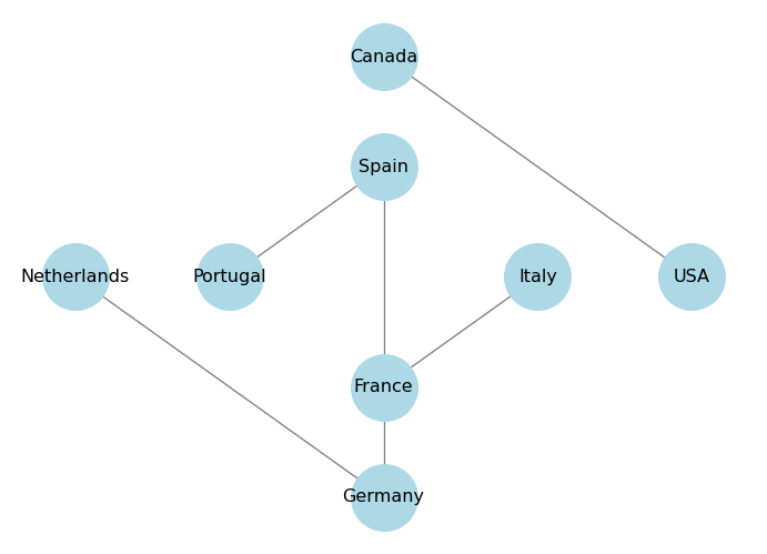

What’s Next?

The next page uses colours, sizes and labels to show node and edge attributes.

Drawing Attributes