SIR Simulation

Module 5: Complex Networks

This page continues SIR on Networks. The first chunk repeats the parameters, the graph and the initial state.

import matplotlib.pyplot as plt
import networkx as nx
import numpy as np

SEED = 7
beta = 0.20
mu = 0.10
steps = 120
initial_infected = 5
N = 100


def make_graph(model: str, n: int, seed: int = SEED):
    if model == "random":
        return nx.erdos_renyi_graph(n=n, p=6 / (n - 1), seed=seed)
    if model == "small-world":
        return nx.watts_strogatz_graph(n=n, k=6, p=0.08, seed=seed)
    if model == "scale-free":
        return nx.barabasi_albert_graph(n=n, m=3, seed=seed)
    raise ValueError("model must be one of: 'random', 'small-world', 'scale-free'")


def initialize_state(G, initial_infected=5, seed: int = SEED):
    rng = np.random.default_rng(seed)
    infected = rng.choice(list(G.nodes()), size=initial_infected, replace=False)
    state = {node: ("I" if node in infected else "S") for node in G.nodes()}
    nx.set_node_attributes(G, state, "state")
    return G


G = make_graph("random", n=N, seed=SEED)

Implement the SIR Dynamics

The update is synchronous: compute all changes from the old state, then apply them.

Exercise

Write step_sir(G, beta, mu), one synchronous step of the SIR update. It differs from step_sis in one place: an infected node that recovers moves to “R”, and “R” nodes never change.

def step_sir(G, beta, mu):
    # TODO: read current states from G.nodes[u]["state"]
    # TODO: build new_state dict with values in {"S","I","R"}
    # TODO: write new_state back via nx.set_node_attributes
    return G

Solution

def step_sir(G, beta, mu):
    current = {u: G.nodes[u]["state"] for u in G.nodes()}
    new_state = current.copy()

    for u in G.nodes():
        if current[u] == "S":
            m = sum(1 for v in G.neighbors(u) if current[v] == "I")
            if m > 0:
                p_infect = 1 - (1 - beta) ** m
                if np.random.random() < p_infect:
                    new_state[u] = "I"

        elif current[u] == "I":
            if np.random.random() < mu:
                new_state[u] = "R"

        else:
            # "R" stays "R"
            pass

    nx.set_node_attributes(G, new_state, "state")
    return G

Exercise

Wrap step_sir into a simulator. Compared to SIS, you track all three counts: \(S(t), I(t), R(t)\). Stop early when no node is infected, since nothing can change after that.

def run_sir(G, beta, mu, steps=100, initial_infected=5, seed=SEED):
    # TODO
    return S_counts, I_counts, R_counts

Solution

def run_sir(G, beta, mu, steps=100, initial_infected=5, seed=SEED):
    H = G.copy()

    # Make the whole run reproducible (step_sir uses np.random.random)
    np.random.seed(seed)

    initialize_state(H, initial_infected=initial_infected, seed=seed)

    def counts(H):
        S = sum(H.nodes[u]["state"] == "S" for u in H.nodes())
        I = sum(H.nodes[u]["state"] == "I" for u in H.nodes())
        R = sum(H.nodes[u]["state"] == "R" for u in H.nodes())
        return S, I, R

    S0, I0, R0 = counts(H)
    S_counts = [S0]
    I_counts = [I0]
    R_counts = [R0]

    for _ in range(steps):
        if I_counts[-1] == 0:
            break
        step_sir(H, beta=beta, mu=mu)
        S, I, R = counts(H)
        S_counts.append(S)
        I_counts.append(I)
        R_counts.append(R)

    return S_counts, I_counts, R_counts

Run and Visualize

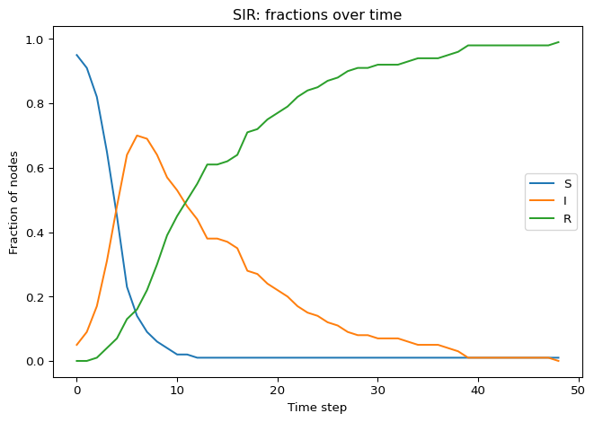
The “epidemic curve” in SIR typically shows a single peak in \(I(t)\) and then decay to zero.

Figure 1: SIR epidemic curve (fractions of S, I, R over time) on one network realization.

Key Questions to Answer

Here are two precise, testable questions that are specific to SIR:

• Can the network become fully infected? That is, does there exist a time \(t\) such that \(I(t)=N\)?
• Can the network become fully “healed”? That is, does there exist a time \(t\) such that \(I(t)=0\)?

In SIR, the second question has a clean answer:

• Yes. For a finite graph with \(\mu>0\), you eventually reach \(I(t)=0\) and then you are stuck forever (absorbing state).

The first question depends on \((\beta,\mu)\) and the network. It can happen transiently, but it is not an absorbing state.

Exercise

Answer these questions, using Figure 1 and your own runs:

• In SIR, is “fully healed” the same as “everyone is susceptible again”? Why not?
• What does “final epidemic size” mean here? (Hint: look at \(R(\infty)\).)
• Can you have an epidemic with a large peak but small final size? Or vice versa?
• Compare two graphs with the same \(N\) and similar average degree: which features (hubs, clustering, path length) do you expect to increase \(R(\infty)\)?

Solution

• No. When \(I = 0\) every node is either S or R. The recovered nodes stay immune, so the network does not return to its initial state. In SIS, by contrast, \(I = 0\) means everyone is susceptible again.
• The final epidemic size is \(R(\infty)/N\), the fraction of nodes that were ever infected, including the initial ones. You read it from the last value of the R curve once \(I = 0\).
• A large peak with a small final size is impossible: every node that is infected at the peak ends in R, so \(R(\infty) \ge \max_t I(t)\). The reverse is possible. On a ring or a lattice with few shortcuts the infection travels as a slow front: only a few nodes are infected at any time, but the front can eventually reach most of the network.
• Hubs and short paths increase \(R(\infty)\). The SIR threshold \(T_c = \langle k \rangle / (\langle k^2 \rangle - \langle k \rangle)\) decreases when the degree distribution is broader (newman2002spread?), and short paths let the outbreak reach distant parts of the network before it dies out. High clustering tends to decrease \(R(\infty)\), because many infection attempts hit neighbours that are already infected or recovered.

What’s Next?

Compare SIS and SIR: how does permanent immunity change the long-run outcome? The next page asks when an epidemic can spread at all.

Epidemic Threshold