SIS Simulation on Networks

Module 5: Complex Networks

This page continues SIS Initial State. The first chunk repeats the parameters and the helper functions you wrote on the previous two pages.

import matplotlib.pyplot as plt
import networkx as nx
import numpy as np

SEED = 7
beta = 0.20  # infection probability per infected neighbour (per step)
mu = 0.10    # recovery probability (per step)
steps = 120
initial_infected = 5
N = 100


def make_graph(model: str, n: int, seed: int = SEED):
    if model == "random":
        return nx.erdos_renyi_graph(n=n, p=6 / (n - 1), seed=seed)
    if model == "small-world":
        return nx.watts_strogatz_graph(n=n, k=6, p=0.08, seed=seed)
    if model == "scale-free":
        return nx.barabasi_albert_graph(n=n, m=3, seed=seed)
    raise ValueError("model must be one of: 'random', 'small-world', 'scale-free'")


def initialize_state(G, initial_infected=5, seed=SEED, rng=None):
    if rng is None:
        rng = np.random.default_rng(seed)
    nx.set_node_attributes(G, "S", "state")
    infected = rng.choice(list(G.nodes()), size=initial_infected, replace=False)
    for node in infected:
        G.nodes[node]["state"] = "I"
    return G


G = make_graph("random", n=N)

Implement the SIS dynamics

The update is synchronous: compute all changes from the old state, then apply them.

Exercise

Create a function step_sis(<graph>, beta, mu) that performs one step of the SIS update. Remember that beta is the infection probability and mu is the recovery probability.

def step_sis(G, beta, mu):
    # TODO: read current states from G.nodes[u]["state"]
    # TODO: compute a new_state mapping (synchronous update)
    # TODO: write new_state back to node attributes
    return G

Hint

Loop through all nodes and their neighbours with G.nodes() and G.neighbors(node). Use a random number generator such as np.random.default_rng() for the probabilistic transitions.

Solution

def step_sis(G, beta, mu, rng=None):
    if rng is None:
        rng = np.random.default_rng()

    # Retrieve current states of all nodes
    current = {node: G.nodes[node]["state"] for node in G.nodes()}
    new_state = current.copy()  # start with the same state for synchronous update
    # Loop through all nodes to compute new states
    for node in G.nodes():
        if current[node] == "S":
            # Count infected neighbors
            m = sum(1 for nbr in G.neighbors(node) if current[nbr] == "I")
            if m > 0:
                # Compute infection probability
                p_infect = 1 - (1 - beta) ** m
                if rng.random() < p_infect:
                    new_state[node] = "I"
        else:  # current[node] == "I"
            if rng.random() < mu:
                new_state[node] = "S"
    nx.set_node_attributes(G, new_state, "state")
    return G

Exercise

Wrap step_sis into a simulator that records the number of infected nodes over time. The function run_sis() should take a graph and the parameters, run the simulation for a given number of steps, and return a list of the number of infected nodes at each time step.

def run_sis(G, beta, mu, steps=100, initial_infected=5, seed=SEED):
    # TODO
    return infected_counts

Solution

Copy the graph so that the original stays untouched, and let one seeded generator control all the randomness of a run.

def run_sis(G, beta, mu, steps=100, initial_infected=5, seed=SEED):
    # Copy the graph to avoid mutating the original
    H = G.copy()

    # One seeded RNG controls all randomness for this run
    rng = np.random.default_rng(seed)

    # Initialize states
    initialize_state(H, initial_infected=initial_infected, seed=seed, rng=rng)
    # Count initial number of infected nodes and initialize the list
    infected_counts = [sum(H.nodes[node]["state"] == "I" for node in H.nodes())]
    # Apply SIS steps and record infected counts
    for _ in range(steps):
        step_sis(H, beta=beta, mu=mu, rng=rng)
        infected_counts.append(sum(H.nodes[node]["state"] == "I" for node in H.nodes()))
    return infected_counts

Execute the function to make sure it runs without errors and returns a reasonable output:

counts = run_sis(G, beta=beta, mu=mu, steps=steps, initial_infected=initial_infected)
print("Infected counts over time:", counts)

Infected counts over time: [5, 13, 24, 36, 60, 72, 77, 84, 89, 87, 90, 77, 85, 87, 83, 87, 88, 84, 90, 85, 86, 89, 85, 88, 84, 82, 93, 89, 87, 87, 89, 80, 86, 82, 84, 83, 82, 89, 90, 84, 92, 84, 91, 83, 80, 89, 84, 83, 88, 86, 92, 87, 85, 85, 80, 86, 87, 85, 89, 89, 88, 91, 94, 89, 89, 90, 86, 85, 87, 91, 92, 88, 85, 90, 85, 84, 84, 88, 91, 82, 85, 82, 87, 84, 83, 85, 81, 84, 85, 89, 87, 85, 81, 87, 86, 88, 87, 88, 81, 86, 86, 79, 88, 85, 84, 86, 84, 88, 89, 87, 93, 92, 87, 92, 90, 89, 88, 89, 78, 84, 87]

Validation

Test the code on a case you can solve by hand. With \(\beta = 0\) nobody gets infected, and each infected node recovers with probability \(\mu\) per step. The expected number of infected nodes is \(I(t) = I(0)(1-\mu)^t\).

runs_check = [run_sis(G, beta=0.0, mu=mu, steps=30, initial_infected=50, seed=SEED + r) for r in range(20)]
mean_check = np.mean(runs_check, axis=0)
for t in [0, 10, 20, 30]:
    print(f"t = {t:2d}: simulated {mean_check[t]:5.1f}, expected {50 * (1 - mu) ** t:5.1f}")

t =  0: simulated  50.0, expected  50.0
t = 10: simulated  16.8, expected  17.4
t = 20: simulated   6.0, expected   6.1
t = 30: simulated   2.4, expected   2.1

Run and Visualize

Exercise

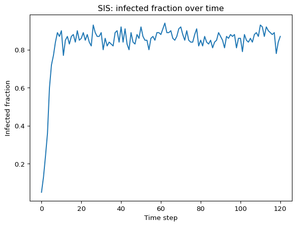
Use matplotlib to plot the fraction of infected nodes over time for one run of run_sis on G. Try to get a graph similar to Figure 1 below.

Figure 1: Fraction of infected nodes over time for a single SIS run on a random graph.

Solution

Divide the counts by the number of nodes to get a fraction.

counts = run_sis(G, beta=beta, mu=mu, steps=steps, initial_infected=initial_infected, seed=SEED)
plt.plot(np.array(counts) / G.number_of_nodes())
plt.xlabel("Time step")
plt.ylabel("Infected fraction")
plt.title("SIS: infected fraction over time")
plt.show()

What’s Next?

The next page compares the three network types.

Comparing Networks under SIS