Swing Equation
Module 5: Complex Networks
The Motter-Lai model has no dynamics. A common next step in power grid modelling describes each node by a phase that obeys the swing equation, a Kuramoto model with inertia (filatrella2008analysis?; schafer2018dynamically?). You met the first-order Kuramoto model in The Kuramoto Model.
The model
Each node \(i\) is a generator (\(P_i > 0\)) or a consumer (\(P_i < 0\)). Its phase \(\theta_i\) is measured in a frame that rotates at the grid reference frequency (50 Hz in Europe). The swing equation reads
\[ M \ddot{\theta}_i + D \dot{\theta}_i = P_i + \sum_{j} K_{ij} \sin(\theta_j - \theta_i), \]
where \(M\) is the inertia, \(D\) the damping and \(K_{ij}\) the capacity of the line between \(i\) and \(j\) (\(K_{ij} = 0\) if there is no line) (filatrella2008analysis?). The power flow on line \((i,j)\) is \(F_{ij} = K_{ij}\sin(\theta_j - \theta_i)\).
- With \(M = 0\) you recover the first-order Kuramoto model, with natural frequencies \(P_i / D\).
- A synchronous state has \(\dot{\theta}_i = 0\) for all \(i\) in the rotating frame. It requires \(\sum_i P_i = 0\) (supply equals demand) and lines strong enough to carry the flows.
Dynamical cascades
(schafer2018dynamically?) combine the swing equation with a line-failure rule: a line fails when the magnitude of its flow exceeds a threshold. When one line fails, the flows reroute through a transient that lasts seconds. During the transient a flow can overshoot its new steady-state value and trip a line that a static calculation would call safe. This mechanism is absent from any static model such as Motter-Lai.
A two-node example
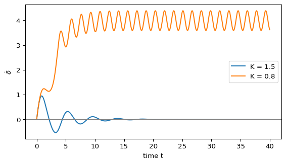
Take one generator with \(P_1 = P\) and one consumer with \(P_2 = -P\), joined by one line of capacity \(K\). Subtract the two equations. The phase difference \(\delta = \theta_1 - \theta_2\) obeys
\[ M \ddot{\delta} + D \dot{\delta} = 2P - 2K \sin\delta . \]
A fixed point needs \(\sin\delta^* = P/K\), so it exists only if \(K \ge P\). The line must be able to carry the power. Figure 1 integrates the equation for \(K\) above and below this bound.
Exercise
Find the fixed points of the two-node equation for \(K = 2P\) and decide which one is stable.
Solution
\(\sin\delta^* = 1/2\) gives \(\delta^* = \pi/6\) and \(\delta^* = 5\pi/6\). Linearize: \(M\ddot{u} + D\dot{u} + 2K\cos(\delta^*)\,u = 0\). At \(\pi/6\) the restoring term is positive, so the fixed point is stable (a damped oscillation). At \(5\pi/6\) it is negative, so the fixed point is a saddle.
Optional extension
Build a ring of 6 nodes with alternating \(P_i = \pm 1\) and equal \(K\). Integrate the swing equation with solve_ivp and find numerically the smallest \(K\) for which the ring synchronizes. Then remove one line and repeat.
Exit question
The official report on the Iberian blackout lists voltage control, oscillations and generator disconnections among the interacting factors (entsoe2026final?). Name one of these factors that the swing equation can represent and one that neither the swing equation nor the Motter-Lai model can represent.
Answer
The swing equation describes phase angles and frequency, so it can produce oscillations, such as the damped oscillation around a stable fixed point in the exercise above. Neither model has voltage magnitudes or reactive power, so neither can represent a voltage rise or the overvoltage disconnections that the report describes.