Dispersion Relation
Module 4: Space and Pattern Formation
The Turing conditions tell you whether some mode grows. The dispersion relation tells you which modes grow and how fast (murray2003mathematical? and 2.6).
Growth Rate Versus Wavenumber
For each wavenumber \(k\), the growth rates are the roots of
\[ \sigma^2 - \operatorname{tr}A(k^2)\,\sigma + h(k^2) = 0, \qquad A(k^2) = \gamma J - k^2\operatorname{diag}(1, d), \tag{1}\]
with \(h(k^2) = \det A(k^2) = d\,k^4 - \gamma (d f_u + g_v) k^2 + \gamma^2 \det J\), as on the Turing Conditions page. The function \(k \mapsto \operatorname{Re}\sigma(k^2)\), taking the larger root, is the dispersion relation.
The Unstable Band
\(\sigma > 0\) exactly when \(h(k^2) < 0\). The roots of \(h\) give the band
\[ k_1^2 < k^2 < k_2^2, \qquad k_{1,2}^2 = \frac{\gamma}{2d}\left[(d f_u + g_v) \mp \sqrt{(d f_u + g_v)^2 - 4 d \det J}\right]. \tag{2}\]
The band has width proportional to \(\gamma\) in \(k^2\). At \(d = d_c\) it shrinks to the single value \(k_c^2 = \gamma (d_c f_u + g_v)/(2 d_c)\) (murray2003mathematical?).
The Fastest-Growing Mode
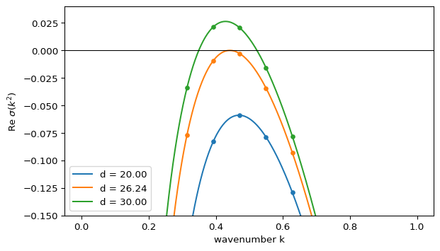
The fastest-growing wavenumber \(k_{\max}\) maximizes \(\operatorname{Re}\sigma(k^2)\). Near onset it is close to \(k_m\), the minimizer of \(h\), but the two are not equal in general, because \(\sigma\) also depends on the trace. You find \(k_{\max}\) numerically. The corresponding wavelength \(2\pi/k_{\max}\) predicts the spacing of the first visible pattern. Nonlinear effects can change the spacing later (murray2003mathematical?).
On a finite domain only discrete wavenumbers exist. With Neumann conditions on \((0, L)\), \(k_n = n\pi/L\). The mode that grows fastest is the admissible \(k_n\) with the largest \(\sigma\). If no \(k_n\) falls into the band, the uniform state stays stable even when the Turing conditions hold.
For \(d = 20\) every mode decays. At \(d = d_c \approx 26.24\) the curve touches zero. For \(d = 30\) a band of modes grows.
import numpy as np

from amlab.turing import dispersion_relation, gierer_meinhardt_jacobian, unstable_band

jac = gierer_meinhardt_jacobian(0.40, 1.00)
d = 30
k1_sq, k2_sq = unstable_band(*jac, d)
k = np.linspace(np.sqrt(k1_sq), np.sqrt(k2_sq), 2001)
k_max = k[np.argmax(dispersion_relation(k**2, *jac, d))]

print(f"unstable band: {np.sqrt(k1_sq):.3f} < k < {np.sqrt(k2_sq):.3f}")
print(f"fastest-growing k = {k_max:.3f}, wavelength = {2 * np.pi / k_max:.1f}")
print(f"closest Neumann mode on L = 40: n = {k_max * 40 / np.pi:.2f}")
unstable band: 0.349 < k < 0.523
fastest-growing k = 0.429, wavelength = 14.6
closest Neumann mode on L = 40: n = 5.46The fastest wavenumber \(k_{\max} \approx 0.43\) corresponds to a wavelength of about \(14.6\), which lies between the Neumann modes \(n = 5\) and \(n = 6\) on \(L = 40\). Both modes grow, at almost the same rate, and mode \(5\) is slightly faster. The laboratory checks which one the simulation selects.
Exercise
Keep \(d = 30\) and \(\gamma = 1\) with Neumann conditions. Mode \(n\) is unstable when \(k_1 < n\pi/L < k_2\). For which domain lengths \(L < 20\) is no mode \(n \ge 1\) unstable?
Solution
The code above gives \(k_1 \approx 0.349\) and \(k_2 \approx 0.523\). Mode \(n\) is unstable for \(n\pi/k_2 < L < n\pi/k_1\):
- \(n = 1\): \(6.01 < L < 8.99\),
- \(n = 2\): \(12.02 < L < 17.99\),
- \(n = 3\): \(18.03 < L < 26.98\).
No mode is unstable for \(L \le 6.01\), for \(8.99 \le L \le 12.02\), and in the narrow gap \(17.99 \le L \le 18.03\). Beyond that the intervals overlap. Small domains and some intermediate sizes stay uniform even though the Turing conditions hold (murray2003mathematical?).