Flows on the Circle
Module 2: Synchronization and Collective Behaviour
A periodic rhythm can be described by a single angle, the phase \(\theta\). The phase lives on the circle: \(\theta\) and \(\theta + 2\pi\) are the same state. A one-dimensional flow on the circle is
\[ \dot\theta = f(\theta), \qquad f(\theta + 2\pi) = f(\theta). \tag{1}\]
Unlike a flow on the line, a flow on the circle can return to its starting point. This is the simplest model of an oscillator (Strogatz 2024, sec. 4.1).
Uniform oscillator
The simplest choice is a constant speed, \(\dot\theta = \omega\). The solution is \(\theta(t) = \omega t + \theta_0\) and the period is \(T = 2\pi/\omega\) (Strogatz 2024, sec. 4.2).
Nonuniform oscillator
A phase that speeds up and slows down along the cycle obeys
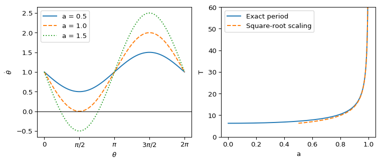
\[ \dot\theta = \omega - a \sin\theta, \qquad \omega > 0,\; a \ge 0. \tag{2}\]
This equation appears in the firefly model, in overdamped pendulums and in Josephson junctions (Strogatz 2024, sec. 4.3 to 4.6). Its behaviour depends on the ratio \(a/\omega\).
- For \(a < \omega\) there are no fixed points. The phase circulates, slowest near \(\theta = \pi/2\).
- At \(a = \omega\) a half-stable fixed point appears at \(\theta = \pi/2\). This is a saddle-node bifurcation on the circle (see Saddle-Node Bifurcation).
- For \(a > \omega\) there are two fixed points with \(\sin\theta^* = \omega/a\). One is stable and one is unstable. The oscillation stops.
For \(a < \omega\) the period is
\[ T = \int_0^{2\pi} \frac{d\theta}{\omega - a\sin\theta} = \frac{2\pi}{\sqrt{\omega^2 - a^2}}. \tag{3}\]
As \(a \to \omega^-\) the period diverges like \(T \approx \dfrac{\sqrt{2}\,\pi}{\sqrt{\omega}}\,(\omega - a)^{-1/2}\). The trajectory spends almost all its time in the bottleneck left behind by the fixed points that are about to appear (Strogatz 2024, sec. 4.3).
Exercise
Take \(a > \omega\). Find the two fixed points of Equation 2 in \([0, 2\pi)\) and decide which one is stable.
Solution
The fixed points satisfy \(\sin\theta^* = \omega/a < 1\), so \(\theta_1^* = \arcsin(\omega/a) \in (0, \pi/2)\) and \(\theta_2^* = \pi - \theta_1^*\). The derivative of the vector field is \(f'(\theta) = -a\cos\theta\). At \(\theta_1^*\) the cosine is positive, so \(f' < 0\) and the point is stable. At \(\theta_2^*\) the cosine is negative and the point is unstable.
Exercise
Check Equation 3 numerically for \(\omega = 1\) and \(a = 0.8\). Integrate the ODE with solve_ivp and measure the time it takes \(\theta\) to grow by \(2\pi\).
Solution
The formula gives \(T = 2\pi/\sqrt{1 - 0.64} = 2\pi/0.6 \approx 10.47\).
import numpy as np
from scipy.integrate import solve_ivp

def rhs(t, theta, omega, a):
    return omega - a * np.sin(theta)

def one_turn(t, theta, omega, a):
    return theta[0] - 2 * np.pi

one_turn.terminal = True
sol = solve_ivp(rhs, (0, 100), [0.0], args=(1.0, 0.8), events=one_turn, rtol=1e-10)
print(sol.t_events[0][0])  # about 10.472
References
Strogatz, Steven H. 2024. Nonlinear Dynamics and Chaos: With Applications to Physics, Biology, Chemistry, and Engineering. Chapman; Hall/CRC.