Saddle-Node Bifurcation
Module 1: Low-Dimensional Dynamics
Reading
- Compulsory: Strogatz (2024), Section 3.7.
- Recommended: (murray2002mathematical?), Chapter 1 (continuous population models for single species).
A bifurcation is a qualitative change in the dynamics as a parameter crosses a critical value: fixed points appear, disappear or change stability. In one dimension, the basic way to create or destroy fixed points is the saddle-node bifurcation (Strogatz 2024, sec. 3.1).
Normal form
The prototype is
\[ \dot x = \mu + x^2 . \tag{1}\]
- \(\mu < 0\): two fixed points \(x^* = \pm\sqrt{-\mu}\). The negative one is stable, the positive one unstable.
- \(\mu = 0\): one half-stable fixed point at \(x^* = 0\).
- \(\mu > 0\): no fixed points.
As \(\mu\) increases through 0, the two fixed points approach each other, collide and annihilate. Near any saddle-node bifurcation of a smooth 1D system, a Taylor expansion reduces the dynamics to Equation 1, which is why it is called a normal form (Strogatz 2024, sec. 3.1).
Conditions
At a saddle-node bifurcation of \(\dot x = f(x; \mu)\), a fixed point is also a point of tangency:
\[ f(x^*; \mu_c) = 0, \qquad \frac{\partial f}{\partial x}(x^*; \mu_c) = 0 . \tag{2}\]
The linearization gives no information at \(\mu_c\): the decay rate \(|f'(x^*)|\) goes to zero, and perturbations relax more and more slowly as \(\mu \to \mu_c\). This is called critical slowing down.
Bifurcation diagram of the budworm
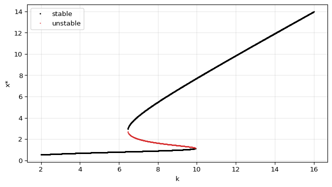
Apply Equation 2 to the budworm model with \(k\) as the control parameter and \(r = 0.56\) fixed. Figure 1 plots the positive fixed points against \(k\).
The diagram has an S shape. The middle branch is unstable. At each fold, a stable branch meets the unstable branch in a saddle-node bifurcation.
You can find the folds numerically by checking where the number of equilibria changes:
counts = [len(budworm_equilibria(0.56, k)) for k in np.linspace(2, 16, 1400)]
k_grid = np.linspace(2, 16, 1400)
changes = k_grid[1:][np.diff(counts) != 0]
print("Number of equilibria changes near k =", np.round(changes, 2))
Number of equilibria changes near k = [6.45 9.94]
Exercise
Show that the saddle-node conditions Equation 2 for \(f(x) = rx(1 - x/k) - x^2/(1+x^2)\) can be solved for \(r\) and \(k\) in terms of the double root \(x\).
Solution
For \(x \neq 0\) divide \(f = 0\) by \(x\): \(r(1 - x/k) = x/(1+x^2)\). Tangency of the two curves means equal slopes: \(-r/k = (1 - x^2)/(1 + x^2)^2\). Substituting \(r/k\) into the first equation gives
\[ r = \frac{2x^3}{(1 + x^2)^2}, \qquad k = \frac{2x^3}{x^2 - 1}, \qquad x > 1, \]
as in Strogatz (2024), Section 3.7. These curves are used on the next page.
Next
Strogatz, Steven H. 2024. Nonlinear Dynamics and Chaos: With Applications to Physics, Biology, Chemistry, and Engineering. Chapman; Hall/CRC.