Kuramoto Lab: Bifurcation Diagram
Module 2: Synchronization and Collective Behaviour
This page is the experiment step. You scan the coupling \(K\), measure the steady-state coherence \(r_\infty\) and compare it with theory. As \(K\) increases, the system moves from incoherence (\(r \approx 0\)) to partial synchrony (\(r > 0\)) (Kuramoto 2003; Strogatz 2000).
Theory to compare with
For any symmetric unimodal frequency density \(g(\omega)\), the critical coupling is (Critical Coupling)
\[ K_c = \frac{2}{\pi g(0)}. \tag{1}\]
For a Cauchy (Lorentzian) distribution with scale parameter \(\gamma\),
\[ g(\omega)=\frac{1}{\pi} \frac{\gamma}{\omega^2+\gamma^2}, \tag{2}\]
so \(g(0)=1/(\pi\gamma)\) and the critical coupling simplifies to
\[ K_c = 2\gamma. \tag{3}\]
In this case the order parameter has a closed form:
\[ r_\infty(K)= \begin{cases} 0, & K \le K_c, \\ \sqrt{1-\frac{K_c}{K}}, & K > K_c. \end{cases} \tag{4}\]
Warning: Equation 4 holds only for the Cauchy distribution.
For any other smooth symmetric density with \(g''(0) < 0\), the theoretical order parameter near onset is (Strogatz 2000)
\[ r \approx \sqrt{\frac{16}{\pi K_c^3}} \sqrt{\frac{\mu}{-g''(0)}} \tag{5}\]
where \(\mu\) measures the distance from the critical point (a dimensionless reduced coupling) and \(g''(0)\) is the second derivative of the frequency distribution at \(0\).
\[ \mu = \frac{K - K_c}{K_c} \tag{6}\]
This formula comes from expanding the self-consistency equation for small \(r\). It captures the square-root growth of \(r\) just above \(K_c\) and fails far from it.
For a normal distribution with standard deviation \(\sigma\):
\[ g(\omega) = \frac{1}{\sqrt{2\pi}\sigma} \exp\left(-\frac{\omega^2}{2\sigma^2}\right) \tag{7}\]
\[ g''(\omega) = \left( \frac{\omega^2}{\sigma^4} - \frac{1}{\sigma^2} \right) g(\omega) \tag{8}\]
Experiment
Exercise
In a new script, draw the theoretical bifurcation diagram Equation 4 for \(0 < K < 5\), with \(\gamma = 1\). On top of it, draw the empirical curve. Use \(N = 1000\) oscillators with normal frequencies, \(\sigma = 1\), integrate up to \(t = 100\), and average \(r(t)\) over the window \(90 \le t \le 100\). Use the final phases for one value of \(K\) as the initial condition for the next. (The figures on this page use \(N = 500\) to render quickly.)
k_values = np.linspace(0.0, 5.0, 20)

# TODO: theoretical curve from the Cauchy formula, with K_c = 2 gamma
r_theory =

theta, omega = initialize_oscillators(1000, sigma=1.0, seed=1)
r_inf = np.zeros_like(k_values)
for idx, k in enumerate(k_values):
    # TODO: integrate kuramoto_ode up to t = 100, evaluating 90 <= t <= 100
    # TODO: compute r(t) in that window and store its mean in r_inf[idx]
    # TODO: continue from the last state
    pass

# TODO: plot r_theory as a line and r_inf as points
Hint
Pass t_eval=np.arange(90, 100, 0.1) to solve_ivp() so that sol.y only holds the times you average over. Then np.abs(np.mean(np.exp(1j * sol.y), axis=0)) gives \(r(t)\) at each of those times.
Solution
import numpy as np
import matplotlib.pyplot as plt
from scipy.integrate import solve_ivp

k_values = np.linspace(0.0, 5.0, 20)

# Theoretical curve for a Cauchy density with gamma = 1
kc = 2.0
r_theory = np.zeros_like(k_values)
above = k_values > kc
r_theory[above] = np.sqrt(1 - kc / k_values[above])

theta, omega = initialize_oscillators(1000, sigma=1.0, seed=1)
r_inf = np.zeros_like(k_values)
for idx, k in enumerate(k_values):
    sol = solve_ivp(
        kuramoto_ode, (0, 100), theta,
        t_eval=np.arange(90, 100, 0.1), args=(omega, k),
    )
    r_t = np.abs(np.mean(np.exp(1j * sol.y), axis=0))
    r_inf[idx] = r_t.mean()
    theta = sol.y[:, -1]  # continue from the last state

fig, ax = plt.subplots(figsize=(7, 4))
ax.plot(k_values, r_theory, color="blue", label="Theoretical (Cauchy)")
ax.plot(k_values, r_inf, "o", color="red", label="Empirical (normal frequencies)")
ax.set_xlabel("Coupling strength (K)")
ax.set_ylabel("Order parameter (r)")
ax.legend()
plt.show()
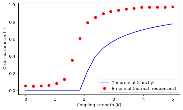
Your plot should look like Figure 1.
Exercise
Do your two curves match? Figure 1 shows a mismatch. Explain why, and fix it.
Solution
The mismatch occurs because the closed-form theoretical curve Equation 4 is derived for a Cauchy frequency distribution, while the empirical data in Figure 1 is generated from a normal distribution.
To fix this you have two consistent options:
- Keep the normal distribution and use a matching theoretical prediction (typically only an approximation near onset, such as Equation 5).
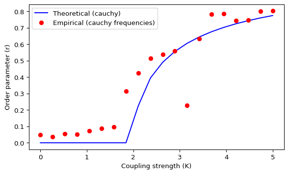
- Keep the closed-form curve Equation 4 and generate the empirical data using a Cauchy distribution.
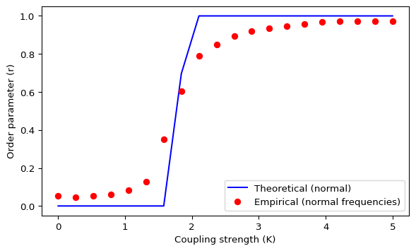
Alternatively, fix the mismatch by changing the empirical distribution to a Cauchy distribution, which matches the closed-form curve Equation 4.
References
Kuramoto, Yoshiki. 2003. Chemical Oscillations, Waves, and Turbulence. Dover Publications.
Strogatz, Steven H. 2000. “From Kuramoto to Crawford: Exploring the Onset of Synchronization in Populations of Coupled Oscillators.” Physica D: Nonlinear Phenomena 143: 1–20.