Linear Systems in the Plane
Module 1: Low-Dimensional Dynamics
Reading
- Compulsory: Strogatz (2024), Chapter 5, Sections 6.1-6.2, Chapter 7 and Section 8.2.
- Recommended: (epstein1998introduction?).
In one dimension a trajectory can only move monotonically towards a fixed point or away from it. In two dimensions it can also rotate, and sustained oscillations become possible. The first step is to understand linear systems, because near a fixed point every smooth system looks linear (Strogatz 2024, chap. 5).
Eigenvalues from trace and determinant
Consider \(\dot{\mathbf x} = A\mathbf x\) with \(A = \begin{pmatrix} a & b \\ c & d \end{pmatrix}\). Let
\[ \tau = \operatorname{tr} A = a + d, \qquad \Delta = \det A = ad - bc . \]
The eigenvalues are the roots of \(\lambda^2 - \tau\lambda + \Delta = 0\):
\[ \lambda_{1,2} = \frac{\tau \pm \sqrt{\tau^2 - 4\Delta}}{2}, \qquad \lambda_1 + \lambda_2 = \tau, \quad \lambda_1\lambda_2 = \Delta . \tag{1}\]
Solutions are combinations of \(e^{\lambda_1 t}\) and \(e^{\lambda_2 t}\), so the signs and the type (real or complex) of the eigenvalues decide the phase portrait (Strogatz 2024, sec. 5.2).
Classification
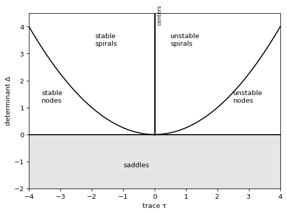
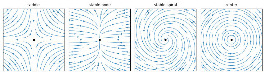
- \(\Delta < 0\): real eigenvalues of opposite sign. Saddle point.
- \(\Delta > 0\) and \(\tau^2 > 4\Delta\): real eigenvalues of the same sign. Node, stable if \(\tau < 0\) and unstable if \(\tau > 0\).
- \(\Delta > 0\) and \(\tau^2 < 4\Delta\): complex eigenvalues \(\tau/2 \pm i\omega\). Spiral, stable if \(\tau < 0\) and unstable if \(\tau > 0\). The frequency is \(\omega = \sqrt{4\Delta - \tau^2}/2\).
- \(\Delta > 0\) and \(\tau = 0\): purely imaginary eigenvalues. Center, with closed orbits.
- \(\Delta = 0\): at least one zero eigenvalue. Non-isolated fixed points.
From linear to nonlinear
For a nonlinear system, the Jacobian at a fixed point plays the role of \(A\). The linear classification carries over to the nonlinear system for saddles, nodes and spirals. Centers and the borderline cases on \(\Delta = 0\) or \(\tau^2 = 4\Delta\) can change type under nonlinear terms (Strogatz 2024, sec. 6.3).
Exercise
Classify the fixed point of \(\dot x = -x + 2y\), \(\dot y = -2x - y\).
Solution
\(\tau = -2\), \(\Delta = 1 + 4 = 5\), \(\tau^2 - 4\Delta = 4 - 20 < 0\). The eigenvalues are \(-1 \pm 2i\): a stable spiral with angular frequency 2.
print(np.linalg.eigvals([[-1, 2], [-2, -1]]))[-1.+2.j -1.-2.j]Next
Strogatz, Steven H. 2024. Nonlinear Dynamics and Chaos: With Applications to Physics, Biology, Chemistry, and Engineering. Chapman; Hall/CRC.