Simulating the SIS Model

Module 1: Low-Dimensional Dynamics

In the SIS model recovered individuals become susceptible again (hethcote2000mathematics?). With \(S = 1 - I\),

\[ \dot I = \beta I (1 - I) - \gamma I . \tag{1}\]

Prediction

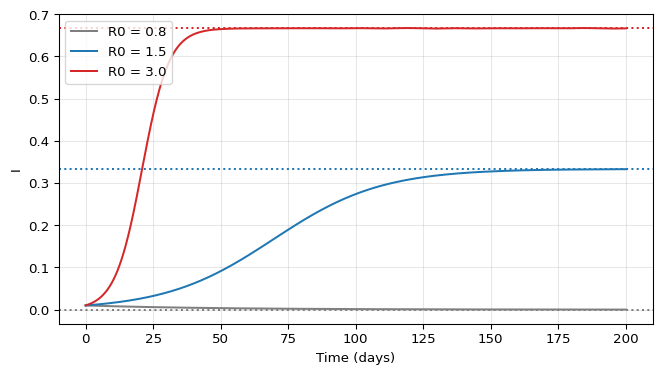
From The Reproduction Number: for \(R_0 = \beta/\gamma > 1\) the solution should approach the endemic level \(I^* = 1 - 1/R_0\); for \(R_0 < 1\) it should decay to 0.

Exercise

Sketch \(\dot I\) against \(I\) for \(R_0 = 2\) and mark the fixed points, as you did for the budworm.

Solution

\(\dot I = I\bigl(\beta(1 - I) - \gamma\bigr)\) is a downward parabola with zeros at \(I = 0\) and \(I^* = 1 - \gamma/\beta = 0.5\). It is positive between them and negative for \(I > 0.5\). So \(I = 0\) is unstable (slope \(\beta - \gamma > 0\)) and \(I^* = 0.5\) is stable (slope \(-(\beta - \gamma) < 0\)).

Implementation

Exercise

Write the right-hand side of Equation 1 in the form solve_ivp expects. The state i arrives as an array with one element.

def sis_model(t, i, beta, gamma):
    didt = # TODO: right-hand side of the SIS equation
    return [didt]

Solution

def sis_model(t, i, beta, gamma):
    return [beta * i[0] * (1 - i[0]) - gamma * i[0]]

The reference version is amlab.epidemics.sis_rhs.

Validation

import matplotlib.pyplot as plt
import numpy as np
from scipy.integrate import solve_ivp

from amlab.epidemics import sis_endemic_level, sis_rhs

gamma = 0.1
t = np.linspace(0, 200, 800)
fig, ax = plt.subplots(figsize=(7, 4))
for r0, color in [(0.8, "tab:gray"), (1.5, "tab:blue"), (3.0, "tab:red")]:
    sol = solve_ivp(sis_rhs, (0, 200), [0.01], args=(r0 * gamma, gamma), t_eval=t)
    ax.plot(sol.t, sol.y[0], color=color, label=f"R0 = {r0}")
    ax.axhline(sis_endemic_level(r0), color=color, ls=":")
    print(f"R0 = {r0}: I(200) = {sol.y[0, -1]:.4f}, 1 - 1/R0 = {sis_endemic_level(r0):.4f}")
ax.set_xlabel("Time (days)")
ax.set_ylabel("I")
ax.legend()
ax.grid(alpha=0.3)
plt.tight_layout()
plt.show()

R0 = 0.8: I(200) = 0.0002, 1 - 1/R0 = 0.0000
R0 = 1.5: I(200) = 0.3328, 1 - 1/R0 = 0.3333
R0 = 3.0: I(200) = 0.6664, 1 - 1/R0 = 0.6667

Figure 1: SIS model with gamma = 0.1 and three values of R0. Dotted lines: endemic level 1 - 1/R0.

Experiment

Exercise

• Start from \(I(0) = 0.9\) with \(R_0 = 1.5\). Does the solution approach the same level from above?
• Take \(R_0\) close to 1, for example 1.05. How long does it take to get close to \(I^*\)? Relate the time scale to the linearization \(f'(I^*) = -(\beta - \gamma)\).

Solution

The endemic equilibrium attracts every \(I(0) > 0\), from above or below. Near it, perturbations decay like \(e^{-(\beta - \gamma)t}\). For \(R_0 = 1.05\) and \(\gamma = 0.1\), \(\beta - \gamma = 0.005\) per day, so the relaxation time is about 200 days.

Interpretation and limitations

The SIS model has no epidemic peak followed by extinction: the disease settles at a constant endemic level. In a finite population the deterministic endemic state hides random fluctuations, and the infection can go extinct by chance when the number of infected individuals is small (Keeling and Rohani 2008).

Optional extension

The SIS equation is a logistic equation. Solve it analytically and compare the formula with the numerical solution.

Next

Keeling, Matt J., and Pejman Rohani. 2008. Modeling Infectious Diseases in Humans and Animals. Princeton University Press.