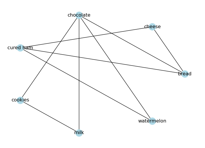
A higher degree centrality means the node is more “important” in terms of connectivity. In the food graph, “chocolate” has the highest degree centrality, while “bread” and “cured ham” are the next most connected nodes.
Closeness Centrality
Closeness measures how close a node is (on average) to all others via shortest paths (Sabidussi 1966). One common definition is
A higher closeness centrality means the node can reach other nodes more quickly. In the food graph, “chocolate” has the highest closeness centrality, followed by “bread”.
Disconnected graphs
If a graph is disconnected, some distances are infinite and closeness becomes tricky. In practice you often compute path-based metrics on the largest connected component.
Betweenness identifies bridges: nodes that sit on many shortest paths (Freeman 1977). Formally,
\[
\mathrm{between}(v) = \sum_{s \neq v \neq t} \frac{\sigma_{st}(v)}{\sigma_{st}},
\]
where \(\sigma_{st}\) is the number of shortest paths from \(s\) to \(t\), and \(\sigma_{st}(v)\) is the number of those paths that pass through \(v\).
bc = nx.betweenness_centrality(G_foods)print("Betweenness centrality:")for node, c insorted(bc.items(), key=lambda kv: kv[1], reverse=True):print(f" {node}: {c:.3f}")
Higher betweenness centrality means the node acts as a bridge between different parts of the graph. In the food graph, “chocolate” has the highest betweenness centrality, with “bread” as the second most important bridge.
PageRank (Directed Networks)
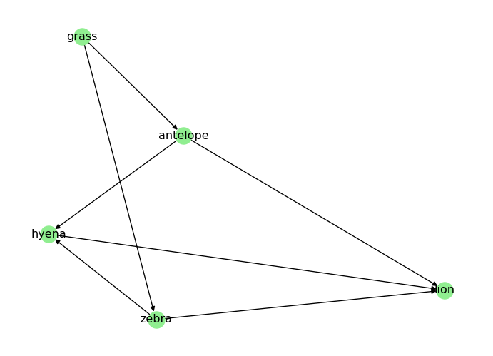
For directed networks (like the web), PageRank is the stationary distribution of a random walk (“random surfer”) on the graph (Page et al. 1999).
Freeman, Linton C. 1977. “A Set of Measures of Centrality Based on Betweenness.”Sociometry 40 (1): 35–41. https://doi.org/10.2307/3033543.
Newman, Mark. 2018. Networks. 2nd ed. Oxford University Press.
Page, Lawrence, Sergey Brin, Rajeev Motwani, and Terry Winograd. 1999. “The PageRank Citation Ranking: Bringing Order to the Web.” 1999-66. Stanford InfoLab. http://ilpubs.stanford.edu:8090/422/.
---title: "Centrality in NetworkX"subtitle: "Module 5: Complex Networks"format: html---::: {.callout-note}## Toolkit pageThis page is self-study material for Session 23. It continues [Degree and Clustering](networkx-degree-clustering.qmd).:::This page ranks nodes with **centrality** measures in `networkx`[@newman2018networks]. You will need betweenness in the cascade lab.You reuse the two graphs from the previous pages.```{python}import networkx as nximport matplotlib.pyplot as plt# Create an undirected graph# (foods that go well together)G_foods = nx.from_edgelist([ ("bread", "cheese"), ("bread", "chocolate"), ("bread", "cured ham"), ("cheese", "cured ham"), ("chocolate", "cookies"), ("chocolate", "milk"), ("chocolate", "watermelon"), ("cookies", "milk"), ("cured ham", "watermelon"),])# Visualize the graphpos = nx.circular_layout(G_foods)nx.draw(G_foods, node_color="lightblue", with_labels=True, pos=pos)plt.show()``````{python}# Create a directed graphD_food_chain = nx.DiGraph() # food chain (prey -> predator)D_food_chain.add_edges_from([ ("grass", "antelope"), ("grass", "zebra"), ("antelope", "lion"), ("antelope", "hyena"), ("zebra", "lion"), ("zebra", "hyena"), ("hyena", "lion"),])# Visualize the graphpos = nx.spring_layout(D_food_chain)nx.draw(D_food_chain, node_color="lightgreen", with_labels=True, pos=pos)plt.show()```## Centrality (Node Importance)In many real networks, not all nodes play the same role:- in an airport network, some airports are **hubs**;- in an email network, some people act as **bridges** between groups.These ideas are quantified by **centrality measures** [@newman2018networks].### Degree CentralityThe simplest centrality is based on degree. In an undirected graph with $N$ nodes, the (normalized) degree centrality is [@newman2018networks]$$\mathrm{deg\_cent}(i) = \frac{k_i}{N-1}.$$```{python}deg_cent = nx.degree_centrality(G_foods)print("Degree centrality:")for node, c insorted(deg_cent.items(), key=lambda kv: kv[1], reverse=True):print(f" {node}: {c:.3f}")```A higher degree centrality means the node is more "important" in terms of connectivity. In the food graph, "chocolate" has the highest degree centrality, while "bread" and "cured ham" are the next most connected nodes.### Closeness CentralityCloseness measures how close a node is (on average) to all others via shortest paths [@sabidussi1966centrality].One common definition is$$\mathrm{close}(i) = \frac{N-1}{\sum_{j \neq i} d(i,j)},$$where $d(i,j)$ is the shortest-path distance.A higher closeness centrality means the node can reach other nodes more quickly. In the food graph, "chocolate" has the highest closeness centrality, followed by "bread".::: {.callout-note}## Disconnected graphsIf a graph is disconnected, some distances are infinite and closeness becomes tricky. In practice you often compute path-based metrics on the **largest connected component**.:::```{python}close_cent = nx.closeness_centrality(G_foods)print("Closeness centrality:")for node, c insorted(close_cent.items(), key=lambda kv: kv[1], reverse=True):print(f" {node}: {c:.3f}")```### Betweenness CentralityBetweenness identifies **bridges**: nodes that sit on many shortest paths [@freeman1977betweenness].Formally,$$\mathrm{between}(v) = \sum_{s \neq v \neq t} \frac{\sigma_{st}(v)}{\sigma_{st}},$$where $\sigma_{st}$ is the number of shortest paths from $s$ to $t$, and $\sigma_{st}(v)$ is the number of those paths that pass through $v$.```{python}bc = nx.betweenness_centrality(G_foods)print("Betweenness centrality:")for node, c insorted(bc.items(), key=lambda kv: kv[1], reverse=True):print(f" {node}: {c:.3f}")```Higher betweenness centrality means the node acts as a bridge between different parts of the graph. In the food graph, "chocolate" has the highest betweenness centrality, with "bread" as the second most important bridge.### PageRank (Directed Networks)For directed networks (like the web), PageRank is the stationary distribution of a random walk ("random surfer") on the graph [@page1999pagerank].```{python}pr = nx.pagerank(D_food_chain, alpha=0.85)print("PageRank (directed food chain):")for node, c insorted(pr.items(), key=lambda kv: kv[1], reverse=True):print(f" {node}: {c:.3f}")```::: {.callout-tip collapse="true"}## Performance noteOn large graphs, exact betweenness can be expensive. NetworkX supports approximation (sample $k$ sources):```pythonnx.betweenness_centrality(G, k=200, seed=SEED)```:::## What's Next?Session 24 uses betweenness as the load of a node in a cascade model.[The Iberian Blackout](iberian-blackout.qmd){.btn .btn-primary}