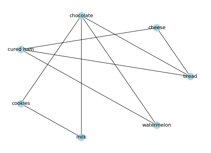
The degree \(k\) of a node is the number of edges connected to it. In an undirected graph, the degree of a node is simply the number of neighbors it has.
# Degree of a nodeprint("Degree of 'bread':", G_foods.degree("bread"))
Degree of 'bread': 3
The average degree of an undirected graph is given by:
\[\langle k \rangle = \frac{2E}{N}\]
where \(E\) is the number of edges and \(N\) is the number of nodes.
# Average degree of the graphls_degrees = [G_foods.degree(node) for node in G_foods.nodes()]avg_degree =sum(ls_degrees) /len(ls_degrees)print("Average degree:", avg_degree)
Average degree: 2.5714285714285716
Degrees in Directed Graphs
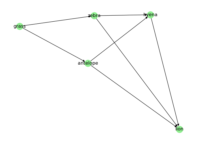
In a directed graph, you distinguish between in-degree (number of incoming edges) and out-degree (number of outgoing edges).
print("In-degree of 'antelope' (number of prey):", D_food_chain.in_degree("antelope"))print("Out-degree of 'antelope' (number of predators):", D_food_chain.out_degree("antelope"))
In-degree of 'antelope' (number of prey): 1
Out-degree of 'antelope' (number of predators): 2
Clustering Coefficient
Many real networks have triangles: if A is connected to B and C, there is a higher-than-random chance that B is also connected to C (Watts and Strogatz 1998; Newman 2018). This tendency is captured by the clustering coefficient.
For an undirected graph, the local clustering coefficient of node \(i\) is:
\[
C_i = \frac{2T_i}{k_i(k_i - 1)}
\]
where \(k_i\) is the degree of node \(i\), and \(T_i\) is the number of triangles that include node \(i\). If \(k_i < 2\), define \(C_i = 0\).
In the food graph, \(C_{\text{bread}} = 1/3\): “bread” has three neighbors, and only one neighbor-pair is connected.
The average clustering coefficient is:
\[
C = \frac{1}{N}\sum_{i=1}^N C_i.
\]
In NetworkX:
nx.clustering(G) returns \(C_i\) for every node.
nx.average_clustering(G) returns the average \(C\).
You will use \(C\) later to compare random vs small-world vs scale-free synthetic networks.
# Local clustering coefficient for each nodeclustering = nx.clustering(G_foods)print("Local clustering:")for node, c in clustering.items():print(f" {node}: {c:.3f}")print("Average clustering:", nx.average_clustering(G_foods))# Another common global measure is transitivity# (ratio of triangles to connected triples)print("Transitivity:", nx.transitivity(G_foods))
Compute the local clustering coefficient of “chocolate” by hand from the drawing of G_foods. Then check your answer with nx.clustering.
Solution
“chocolate” has four neighbours (bread, cookies, milk and watermelon), so there are \(4 \cdot 3 / 2 = 6\) neighbour pairs. Only cookies and milk are connected, so \(C_{\text{chocolate}} = 1/6 \approx 0.167\).
Newman, Mark. 2018. Networks. 2nd ed. Oxford University Press.
Watts, Duncan J., and Steven H. Strogatz. 1998. “Collective Dynamics of ’Small-World’ Networks.”Nature 393 (6684): 440–42. https://doi.org/10.1038/30918.
Source Code
---title: "Degree and Clustering"subtitle: "Module 5: Complex Networks"format: html---::: {.callout-note}## Toolkit pageThis page is self-study material for Session 23. It continues [Paths in Directed Graphs](networkx-directed-paths.qmd).:::This page computes **degree** and **clustering** with `networkx`[@newman2018networks]. You will need degree moments in the epidemic lab.You reuse the two graphs from the previous pages.```{python}import networkx as nximport matplotlib.pyplot as plt# Create an undirected graph# (foods that go well together)G_foods = nx.from_edgelist([ ("bread", "cheese"), ("bread", "chocolate"), ("bread", "cured ham"), ("cheese", "cured ham"), ("chocolate", "cookies"), ("chocolate", "milk"), ("chocolate", "watermelon"), ("cookies", "milk"), ("cured ham", "watermelon"),])# Visualize the graphpos = nx.circular_layout(G_foods)nx.draw(G_foods, node_color="lightblue", with_labels=True, pos=pos)plt.show()``````{python}# Create a directed graphD_food_chain = nx.DiGraph() # food chain (prey -> predator)D_food_chain.add_edges_from([ ("grass", "antelope"), ("grass", "zebra"), ("antelope", "lion"), ("antelope", "hyena"), ("zebra", "lion"), ("zebra", "hyena"), ("hyena", "lion"),])# Visualize the graphpos = nx.spring_layout(D_food_chain)nx.draw(D_food_chain, node_color="lightgreen", with_labels=True, pos=pos)plt.show()```## DegreeThe degree $k$ of a node is the number of edges connected to it. In an undirected graph, the degree of a node is simply the number of neighbors it has.```{python}# Degree of a nodeprint("Degree of 'bread':", G_foods.degree("bread"))```The average degree of an undirected graph is given by:$$\langle k \rangle = \frac{2E}{N}$$where $E$ is the number of edges and $N$ is the number of nodes.```{python}# Average degree of the graphls_degrees = [G_foods.degree(node) for node in G_foods.nodes()]avg_degree =sum(ls_degrees) /len(ls_degrees)print("Average degree:", avg_degree)```### Degrees in Directed GraphsIn a directed graph, you distinguish between in-degree (number of incoming edges) and out-degree (number of outgoing edges).```{python}print("In-degree of 'antelope' (number of prey):", D_food_chain.in_degree("antelope"))print("Out-degree of 'antelope' (number of predators):", D_food_chain.out_degree("antelope"))```## Clustering CoefficientMany real networks have **triangles**: if A is connected to B and C, there is a higher-than-random chance that B is also connected to C [@watts1998collective; @newman2018networks].This tendency is captured by the **clustering coefficient**.For an undirected graph, the *local clustering coefficient* of node $i$ is:$$C_i = \frac{2T_i}{k_i(k_i - 1)}$$where $k_i$ is the degree of node $i$, and $T_i$ is the number of triangles that include node $i$.If $k_i < 2$, define $C_i = 0$.In the food graph, $C_{\text{bread}} = 1/3$: "bread" has three neighbors, and only one neighbor-pair is connected.The **average clustering coefficient** is:$$C = \frac{1}{N}\sum_{i=1}^N C_i.$$In NetworkX:- `nx.clustering(G)` returns $C_i$ for every node.- `nx.average_clustering(G)` returns the average $C$.You will use $C$ later to compare **random** vs **small-world** vs **scale-free** synthetic networks.```{python}# Local clustering coefficient for each nodeclustering = nx.clustering(G_foods)print("Local clustering:")for node, c in clustering.items():print(f" {node}: {c:.3f}")print("Average clustering:", nx.average_clustering(G_foods))# Another common global measure is transitivity# (ratio of triangles to connected triples)print("Transitivity:", nx.transitivity(G_foods))```::: {.callout-note}## ExerciseCompute the local clustering coefficient of "chocolate" by hand from the drawing of `G_foods`. Then check your answer with `nx.clustering`.:::::: {.callout-tip collapse="true"}## Solution"chocolate" has four neighbours (bread, cookies, milk and watermelon), so there are $4 \cdot 3 / 2 = 6$ neighbour pairs. Only cookies and milk are connected, so $C_{\text{chocolate}} = 1/6 \approx 0.167$.```{python}print(nx.clustering(G_foods, "chocolate"))```:::## What's Next?The next page ranks nodes by centrality.[Centrality in NetworkX](networkx-centrality.qmd){.btn .btn-primary}