Comparing Networks under SIS

Module 5: Complex Networks

This page continues SIS Simulation, where you plotted a single run. The first chunk repeats the parameters and all the functions you wrote on the previous pages.

import matplotlib.pyplot as plt
import networkx as nx
import numpy as np

SEED = 7
beta = 0.20  # infection probability per infected neighbour (per step)
mu = 0.10    # recovery probability (per step)
steps = 120
initial_infected = 5
N = 100


def make_graph(model: str, n: int, seed: int = SEED):
    if model == "random":
        return nx.erdos_renyi_graph(n=n, p=6 / (n - 1), seed=seed)
    if model == "small-world":
        return nx.watts_strogatz_graph(n=n, k=6, p=0.08, seed=seed)
    if model == "scale-free":
        return nx.barabasi_albert_graph(n=n, m=3, seed=seed)
    raise ValueError("model must be one of: 'random', 'small-world', 'scale-free'")


def initialize_state(G, initial_infected=5, seed=SEED, rng=None):
    if rng is None:
        rng = np.random.default_rng(seed)
    nx.set_node_attributes(G, "S", "state")
    infected = rng.choice(list(G.nodes()), size=initial_infected, replace=False)
    for node in infected:
        G.nodes[node]["state"] = "I"
    return G

def step_sis(G, beta, mu, rng=None):
    if rng is None:
        rng = np.random.default_rng()
    current = {node: G.nodes[node]["state"] for node in G.nodes()}
    new_state = current.copy()
    for node in G.nodes():
        if current[node] == "S":
            m = sum(1 for nbr in G.neighbors(node) if current[nbr] == "I")
            if m > 0 and rng.random() < 1 - (1 - beta) ** m:
                new_state[node] = "I"
        elif rng.random() < mu:
            new_state[node] = "S"
    nx.set_node_attributes(G, new_state, "state")
    return G


def run_sis(G, beta, mu, steps=100, initial_infected=5, seed=SEED):
    H = G.copy()
    rng = np.random.default_rng(seed)
    initialize_state(H, initial_infected=initial_infected, seed=seed, rng=rng)
    infected_counts = [sum(H.nodes[node]["state"] == "I" for node in H.nodes())]
    for _ in range(steps):
        step_sis(H, beta=beta, mu=mu, rng=rng)
        infected_counts.append(sum(H.nodes[node]["state"] == "I" for node in H.nodes()))
    return infected_counts


G = make_graph("random", n=N)

Compare Network Types

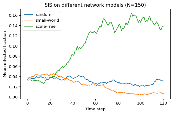
With \(\beta = 0.2\) and \(\langle k \rangle \approx 6\) every network ends up with most nodes infected, so the structure hardly matters. The differences show up closer to the epidemic threshold, so Figure 1 uses \(\beta = 0.02\).

Exercise

Run 12 simulations for each graph type with \(N = 150\) and \(\beta = 0.02\), and plot the average infected fraction over time on the same axes. Use SEED + r for both the graph and the dynamics of run r.

Figure 1: Mean infected fraction over time for three network models with N = 150 and mean degree close to 6 (beta = 0.02, mu = 0.1, 12 runs each).

Solution

models = ["random", "small-world", "scale-free"]
N = 150
runs = 12
beta_compare = 0.02

for model in models:
    trajectories = []
    for r in range(runs):
        seed_run = SEED + r
        Gm = make_graph(model, n=N, seed=seed_run)
        counts = run_sis(Gm, beta=beta_compare, mu=mu, steps=steps,
                         initial_infected=initial_infected, seed=seed_run)
        trajectories.append(np.array(counts) / N)
    plt.plot(np.mean(trajectories, axis=0), label=model)

plt.xlabel("Time step")
plt.ylabel("Mean infected fraction")
plt.legend()
plt.show()

Interpretation

Exercise

Compare Figure 1 with your prediction on SIS Model on Networks:

• Which network type sustains infection longer at the same \((\beta, \mu)\)?
• Do hubs (scale-free) make persistence easier? Why?
• How does clustering (small-world) change local outbreaks vs global spread?
• If you increase \(N\) but keep average degree similar, what do you expect to happen?

Solution

• The scale-free graph. At \(\beta = 0.02\) it keeps close to 20% of its nodes infected, the random graph a few percent and the small-world graph almost none.
• Yes. A hub has many neighbours, so it is reinfected soon after it recovers, and while infected it exposes many susceptible nodes. This is why the threshold \(\langle k \rangle / \langle k^2 \rangle\) of Epidemic Threshold is lower on heterogeneous networks.
• In the small-world graph most neighbours of an infected node are also neighbours of each other. Many infection attempts hit nodes that are already infected, and the outbreak stays local for longer. Only the few rewired shortcuts carry it across the ring.
• With 5 initial infected nodes, a larger \(N\) starts from a smaller infected fraction, so the curves take longer to rise. The long-time prevalence depends on the threshold. For the random and small-world graphs the threshold does not depend on \(N\) at fixed mean degree. For the Barabási-Albert graph \(\langle k^2 \rangle\) grows like \(\ln N\), so its threshold decreases slowly and persistence becomes easier.

Limitations

• Time is discrete and all nodes update at once. The continuous-time SIS model used in the theory of Epidemic Threshold has rates instead of probabilities; for small \(\beta\) and \(\mu\) the two are close.
• The contact network is static. Real contacts change over time.
• Every node has the same \(\beta\) and \(\mu\).
• With \(N = 150\) and 12 runs the curves are noisy, and on a finite network SIS always dies out eventually, although this can take extremely long above the threshold.

Optional extension

Exercise

Replace your loop-based simulator by amlab.networks_spreading.run_sis_fast, which uses a sparse adjacency matrix. Use it to plot the long-time prevalence against \(\beta\) for the three models with \(N = 1000\).

Solution

run_sis_fast returns the infected fraction at every step. Average the last 100 steps of a 500-step run to estimate the long-time prevalence.

from amlab.networks_spreading import run_sis_fast

rng = np.random.default_rng(SEED)
betas = np.linspace(0.005, 0.06, 12)
for model in ["random", "small-world", "scale-free"]:
    G = make_graph(model, n=1000)
    prevalence = [
        np.mean(run_sis_fast(G, b, mu, steps=500, initial_infected=20, rng=rng)[-100:])
        for b in betas
    ]
    plt.plot(betas, prevalence, "o-", label=model)
plt.xlabel("beta")
plt.ylabel("long-time prevalence")
plt.legend()
plt.show()

With \(\mu = 0.1\) the scale-free graph already has a positive prevalence at \(\beta = 0.01\). The random graph needs \(\beta \approx 0.02\) and the small-world graph \(\beta \approx 0.025\). Above \(\beta \approx 0.04\) the three curves are close.

What’s Next?

Try the SIR model and compare how permanent immunity changes the outcome.

SIR on Networks