Turing Space

Module 4: Space and Pattern Formation

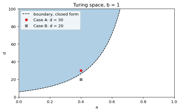
The Turing space is the set of parameters for which the four Turing conditions hold (murray2003mathematical?). For Gierer-Meinhardt you can draw it in the $(a, d)$ plane at fixed $b$.

The Region in Closed Form

From Linearization, the Gierer-Meinhardt Jacobian at the steady state has $f_u = b(1-a)/(1+a)$, $g_v = -1$, and $\det J = b$. The four conditions reduce to:

$\det J = b > 0$, always true.
$\operatorname{tr} J < 0$, that is $f_u < 1$.
$f_u > 0$, that is $a < 1$ (needed for $d f_u + g_v > 0$).
$d f_u - 1 > 2\sqrt{b d}$, which gives

\[ \sqrt{d} > \frac{\sqrt{b} + \sqrt{b + f_u}}{f_u}, \qquad f_u = \frac{b(1-a)}{1+a}. \tag{1}\]

For $b = 1$ the trace condition holds for every $a > 0$, and the Turing space is the region above the curve Equation 1 with $0 < a < 1$.

Figure 1: Turing space of Gierer-Meinhardt for $b = 1$ (shaded), computed with `amlab.pdes_1d.is_turing_instability`. The dashed line is the boundary from Equation 1. The markers are the two test cases of the laboratory.

Reading the Diagram

The curve diverges as $a \to 1$, because $f_u \to 0$ and activation disappears.
For $a = 0.4$ the boundary sits at $d_c \approx 26.24$. Case A lies inside, Case B outside.
The diagram depends only on $a$, $b$ and $d$. It does not depend on $\gamma$ or on the domain. Whether a pattern appears on a given domain also needs an admissible mode in the unstable band (Dispersion Relation).

The same diagram appears in the interactive simulator at bam-applied-math-lab.streamlit.app, where you can click on a point of the $(a, d)$ plane and watch the resulting 1D simulation.

Exercise

Increase $b$ from $1$ to $2$ at $a = 0.4$. Does the critical ratio $d_c$ increase or decrease? Compute it with Equation 1, and check whether the trace condition still holds.

Solution

With $b = 2$, $f_u = 2 \cdot 0.6 / 1.4 = 6/7 \approx 0.857 < 1$, so the trace condition holds. Then $\sqrt{d_c} = (\sqrt 2 + \sqrt{2.857})/0.857 \approx (1.414 + 1.690)/0.857 \approx 3.62$, so $d_c \approx 13.1$. The critical ratio decreases.

import numpy as np
from amlab.turing import critical_diffusion_ratio, gierer_meinhardt_jacobian

print(critical_diffusion_ratio(*gierer_meinhardt_jacobian(a=0.4, b=2.0)))

Next session: Gierer-Meinhardt Model in 1D.

--- title: "Turing Space" subtitle: "Module 4: Space and Pattern Formation" format: html --- The Turing space is the set of parameters for which the four Turing conditions hold [@murray2003mathematical, Section 2.5]. For Gierer-Meinhardt you can draw it in the $(a, d)$ plane at fixed $b$. ## The Region in Closed Form From [Linearization](linearization.qmd), the Gierer-Meinhardt Jacobian at the steady state has $f_u = b(1-a)/(1+a)$, $g_v = -1$, and $\det J = b$. The four conditions reduce to: - $\det J = b > 0$, always true. - $\operatorname{tr} J < 0$, that is $f_u < 1$. - $f_u > 0$, that is $a < 1$ (needed for $d f_u + g_v > 0$). - $d f_u - 1 > 2\sqrt{b d}$, which gives $$ \sqrt{d} > \frac{\sqrt{b} + \sqrt{b + f_u}}{f_u}, \qquad f_u = \frac{b(1-a)}{1+a}. $$ {#eq-ts-boundary} For $b = 1$ the trace condition holds for every $a > 0$, and the Turing space is the region above the curve @eq-ts-boundary with $0 < a < 1$. ```{python} #| label: fig-ts-gm #| fig-cap: 'Turing space of Gierer-Meinhardt for $b = 1$ (shaded), computed with `amlab.pdes_1d.is_turing_instability`. The dashed line is the boundary from @eq-ts-boundary. The markers are the two test cases of the laboratory.' #| fig-width: 7 #| fig-height: 4 #| echo: false import matplotlib.pyplot as plt import numpy as np from amlab.pdes_1d.gierer_meinhardt_1d import is_turing_instability b = 1.00 arr_a = np.linspace(0.005, 0.995, 400) arr_d = np.linspace(0, 100, 400) mesh_a, mesh_d = np.meshgrid(arr_a, arr_d) mask_turing = is_turing_instability(mesh_a, b, mesh_d) fu = b * (1 - arr_a) / (1 + arr_a) d_boundary = ((np.sqrt(b) + np.sqrt(b + fu)) / fu) ** 2 fig, ax = plt.subplots(figsize=(7, 4)) ax.contourf(mesh_a, mesh_d, mask_turing, levels=[0.5, 1.5], colors=["tab:blue"], alpha=0.35) ax.plot(arr_a, d_boundary, "k--", lw=1.2, label="boundary, closed form") ax.plot([0.4], [30], "o", color="tab:red", label="Case A: d = 30") ax.plot([0.4], [20], "s", color="tab:gray", label="Case B: d = 20") ax.set_xlim(0, 1) ax.set_ylim(0, 100) ax.set_xlabel("a") ax.set_ylabel("d") ax.set_title("Turing space, b = 1") ax.legend(loc="upper left") plt.show() plt.close() ``` ## Reading the Diagram - The curve diverges as $a \to 1$, because $f_u \to 0$ and activation disappears. - For $a = 0.4$ the boundary sits at $d_c \approx 26.24$. Case A lies inside, Case B outside. - The diagram depends only on $a$, $b$ and $d$. It does not depend on $\gamma$ or on the domain. Whether a pattern appears on a given domain also needs an admissible mode in the unstable band ([Dispersion Relation](dispersion-relation.qmd)). The same diagram appears in the interactive simulator at [bam-applied-math-lab.streamlit.app](https://bam-applied-math-lab.streamlit.app/Gierer_Meinhardt_1D), where you can click on a point of the $(a, d)$ plane and watch the resulting 1D simulation. ::: {.callout-note} ## Exercise Increase $b$ from $1$ to $2$ at $a = 0.4$. Does the critical ratio $d_c$ increase or decrease? Compute it with @eq-ts-boundary, and check whether the trace condition still holds. ::: ::: {.callout-tip collapse="true"} ## Solution With $b = 2$, $f_u = 2 \cdot 0.6 / 1.4 = 6/7 \approx 0.857 < 1$, so the trace condition holds. Then $\sqrt{d_c} = (\sqrt 2 + \sqrt{2.857})/0.857 \approx (1.414 + 1.690)/0.857 \approx 3.62$, so $d_c \approx 13.1$. The critical ratio decreases. ```python import numpy as np from amlab.turing import critical_diffusion_ratio, gierer_meinhardt_jacobian print(critical_diffusion_ratio(*gierer_meinhardt_jacobian(a=0.4, b=2.0))) ``` ::: Next session: [Gierer-Meinhardt Model in 1D](gierer-meinhardt-1d-model.qmd).