Kuramoto Lab: Locating the Threshold
Module 2: Synchronization and Collective Behaviour
This page is the interpretation step. You compare the transition in your Bifurcation Diagram with the critical coupling \(K_c = 2/(\pi g(0))\) from Critical Coupling.
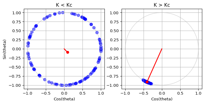
In your animation script from Animation, set the coupling strength just below and just above the critical value to see the difference in the dynamics. Below \(K_c\) the oscillators remain incoherent. Above \(K_c\) they start to synchronize and form a cluster on the unit circle, as in Figure 1.
Exercise
Find \(K_c\) from \(K_c = 2/(\pi g(0))\) for your normal frequencies with \(\sigma = 1\). Estimate the empirical transition point from your points: the value of \(K\) where \(r\) starts to rise clearly above zero. Alternatively, fit the near-onset scaling \(r \approx \sqrt{16/(\pi K_c^3)}\,\sqrt{\mu/(-g''(0))}\) of Bifurcation Diagram to the points just above the transition. Do the two estimates agree?
Solution
For a normal density \(g(0) = 1/\sqrt{2\pi}\), so \(K_c = 2\sqrt{2\pi}/\pi = \sqrt{8/\pi} \approx 1.60\). With \(N = 1000\) and 20 values of \(K\) between 0 and 5, \(r_\infty\) stays below about \(0.1\) up to \(K \approx 1.3\) and jumps to about \(0.6\) between \(K \approx 1.6\) and \(K \approx 1.8\). The grid spacing is about \(0.26\), so the empirical threshold agrees with \(K_c\) within one grid step. The exact \(K\) of the jump moves with the seed, because each sample of frequencies differs from \(g\) (Finite-Size Effects).
Exercise
The empirical points in the normal case lie close to zero for \(K < K_c\) but not exactly at zero. Give two reasons.
Solution
First, a finite population has \(r\) of order \(N^{-1/2}\) even when incoherent (about \(0.045\) for the \(N = 500\) figures of Bifurcation Diagram, \(0.03\) for \(N = 1000\)). Second, the time window may be too short for \(r(t)\) to settle near \(K_c\), where the approach to the steady state is slow. Finite-Size Effects studies the first effect.