Hysteresis
Module 1: Low-Dimensional Dynamics
When a system has an S-shaped bifurcation diagram, the state it occupies depends on the direction in which the parameter changes. This is hysteresis: undoing the change in the parameter does not undo the change in the state (Strogatz 2024, sec. 3.7 and 3.4).
The loop in k
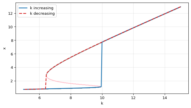
Take \(r = 0.56\) and let \(k\) grow slowly from 5 to 15, then decrease back to 5. “Slowly” means that the population has time to reach the attracting fixed point for each value of \(k\). Figure 1 shows the result on top of the bifurcation diagram from Saddle-Node Bifurcation.
The outbreak starts at \(k \approx 9.94\) but only ends when \(k\) drops below \(6.45\). Between these values the answer to “what is the budworm density for this forest?” depends on history.
The region of bistability
The saddle-node curves from the exercise on the previous page,
\[ r(x) = \frac{2x^3}{(1+x^2)^2}, \qquad k(x) = \frac{2x^3}{x^2 - 1}, \qquad x > 1, \]
bound the region of the \((k, r)\) plane with three positive fixed points (Strogatz 2024, sec. 3.7). The two branches meet at a cusp. Both \(dr/dx\) and \(dk/dx\) vanish at \(x = \sqrt 3\), which gives the cusp point \((k, r) = (3\sqrt 3, 3\sqrt 3/8) \approx (5.20, 0.65)\).
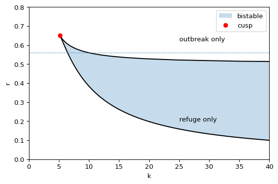
As \(k \to \infty\) the upper curve approaches \(r = 1/2\). Ludwig et al. used this fact: for a large carrying capacity, outbreaks require \(R > 1/2\) in their notation (ludwig1978qualitative?).
Consequences
- An outbreak is triggered by crossing one fold and ended only by crossing the other. Returning the parameter to its value just before the outbreak is not enough.
- Near a fold the refuge state loses resilience: the decay rate \(|f'(x^*)|\) tends to zero, so the system recovers more slowly from perturbations. Similar arguments are used for sudden shifts in lakes, coral reefs and forests (scheffer2001catastrophic?).
Exercise
Fix \(k = 10\) and vary \(r\) instead. The folds are at \(r \approx 0.384\) and \(r \approx 0.560\). Describe what happens when \(r\) increases from 0.3 to 0.7 and then decreases back to 0.3.
Solution
Starting on the refuge branch, the population stays low until \(r \approx 0.560\), where the refuge fixed point disappears and the population jumps to the outbreak level. On the way back it stays high until \(r \approx 0.384\), where the outbreak fixed point disappears and it drops to the refuge. Between 0.384 and 0.560 the state depends on the direction of change.
Optional extension
amlab/odes_1d/spruce_budworm_histeresis.py lets \(k\) oscillate in time, \(k(t) = k_0 + A(1 + \sin 2\pi f t)\), and animates \(x\) against \(k\). Run it locally:
from amlab.odes_1d.spruce_budworm_histeresis import make_animation

make_animation()
Change r inside make_animation to 0.56 and k0, amp so that \(k\) spans the interval \([6, 11]\). Does a loop appear? What happens if you increase the frequency freq?
Next
Strogatz, Steven H. 2024. Nonlinear Dynamics and Chaos: With Applications to Physics, Biology, Chemistry, and Engineering. Chapman; Hall/CRC.